In the previous chapter we started with something complicated.

A continuous field.

A smooth neighborhood.

A growth process.

Localized structures that moved through space.

Patterns that looked disturbingly creature-like.

That was useful because it gave us a mystery.

Now we are going to destroy almost all of it.

Not gradually.

Aggressively.

We want to know:

How little machinery can remain before interesting organization disappears?

Start with the kind of system we saw in Lenia.

Conceptually:

continuous state
+
two-dimensional world
+
large local neighborhood
+
smooth spatial weighting
+
growth response
+
many parameters
+
repeated updates

Now remove things.

Remove continuous state

Instead of allowing every location to contain values such as:

0.00
0.13
0.47
0.81
1.00

allow only:

0
1

Two states.

Nothing in between.

We could call them:

off / on
dead / alive
empty / occupied
white / black

but those names already start smuggling interpretation into the model.

For now:

0
1

is enough.

Remove a dimension

Lenia normally gives us a two-dimensional field.

Remove that too.

Instead of:

0 0 1 0 0
0 1 1 1 0
1 1 0 1 1
0 1 1 1 0
0 0 1 0 0

use a single line:

0 0 0 0 1 0 0 0 0

Our entire world is now one-dimensional.

No creatures can turn north.

There is no north.

No shapes can expand upward.

There is no upward.

Every cell has only a position along a line.

Remove the large neighborhood

Now reduce what each cell can see.

A cell will inspect only:

left
centre
right

Three cells in total.

For the centre cell here:

0 1 1

its entire local universe is:

left   centre   right
  0       1       1

It knows nothing else.

It cannot see ten cells away.

It cannot know what the overall pattern looks like.

It cannot know whether the world contains:

one active cell

or:

a million active cells

unless that difference changes its immediate neighborhood.

This locality is crucial.

Each part has very little information.

Any large-scale organization must arise from repeated interaction.

Remove the complicated response

Lenia uses a smooth response to a neighborhood field.

We don’t need that anymore.

Our cells will use a lookup table.

There are only eight possible three-cell binary neighborhoods:

111
110
101
100
011
010
001
000

For each neighborhood, choose the next state of the centre cell.

For example:

111 → 0
110 → 0
101 → 0
100 → 1
011 → 0
010 → 1
001 → 1
000 → 0

That is an entire rule.

Nothing else is required.

Eight answers define the universe

Because there are eight possible neighborhoods and each can produce either 0 or 1, an elementary rule is completely described by eight bits.

The example above becomes:

00010110

Interpreted as a binary number:

00010110₂ = 22

So this is Rule 22.

The name sounds almost disappointingly mundane.

That’s useful.

We have stripped our system down to:

binary state
+
one-dimensional world
+
three-cell neighborhood
+
eight-bit lookup table

That is almost everything.

Build it

Let’s write the smallest clear implementation.

def step(state, rule):
    next_state = [0] * len(state)

    for i in range(len(state)):
        left = state[(i - 1) % len(state)]
        centre = state[i]
        right = state[(i + 1) % len(state)]

        neighborhood = (left << 2) | (centre << 1) | right
        next_state[i] = (rule >> neighborhood) & 1

    return next_state

There are only two ideas here.

First:

neighborhood = (left << 2) | (centre << 1) | right

turns the three bits into a number from 0 to 7.

For example:

101₂ = 5

Then:

(rule >> neighborhood) & 1

extracts the corresponding output bit from the rule number.

So a number such as:

22

really is enough to encode the entire transition law.

Start with almost nothing

Create a world:

width = 81
state = [0] * width
state[width // 2] = 1

The initial state is:

........................................#........................................

One active cell.

Everything else is zero.

If you prefer numerical form:

00000000000000000000000000000000000000001000000000000000000000000000000000000

This is deliberately austere.

No random initialization.

No hidden state.

No learned parameters.

No population.

No environment.

No organism.

Just one bit.

Let time begin

Now repeat the update:

history = [state]

for _ in range(40):
    state = step(state, rule=22)
    history.append(state)

Every generation becomes a new row.

For display:

for row in history:
    print("".join("#" if cell else "." for cell in row))

The output begins with one active cell.

Then something starts happening.

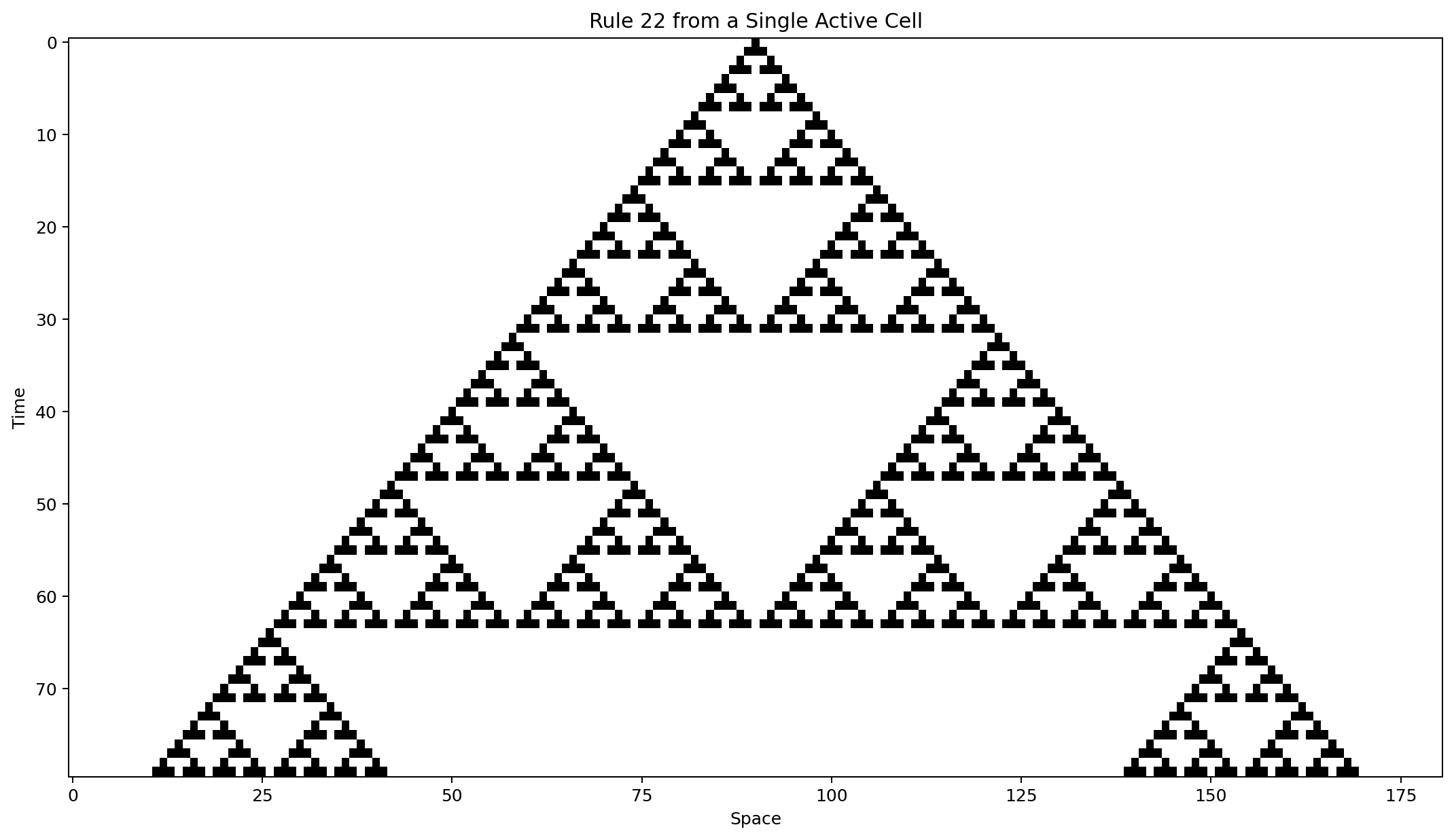
This image is called a spacetime diagram.

Space runs horizontally.

Time runs downward.

One row becomes the next.

The whole history is visible at once.

Nothing is moving downward

This diagram creates a useful illusion.

It looks as though the pattern is falling downward through the image.

It isn’t.

The vertical axis is time.

Each row is the entire world at a different moment.

So:

row 0 = world at t = 0
row 1 = world at t = 1
row 2 = world at t = 2
...

The diagram converts a temporal process into a spatial image.

That technique will appear throughout the book.

It lets us inspect the history of a system instead of watching only its current state.

The update is simultaneous

There is another important detail.

Every cell at time:

t + 1

is computed from the state at:

t

We do not update one cell and allow later cells to see that newly changed value.

Conceptually:

current state
    ↓
compute every next value
    ↓
new state

Not:

change cell 1
    ↓
change cell 2 using modified cell 1
    ↓
change cell 3 using modified cell 2

Those are different models.

A cellular automaton is defined not only by its local rule but also by its update semantics.

We are using synchronous updates.

That means every cell sees the same generation of history.

What happens at the edges?

Our implementation contains this:

state[(i - 1) % len(state)]
state[(i + 1) % len(state)]

The modulo operator makes the world wrap around.

The left edge touches the right edge.

Conceptually:

... 0 1 0 0 1 ...
^                 ^
|_________________|

The line is topologically a ring.

That is not a harmless implementation detail.

We could instead choose:

fixed-zero boundaries
reflective boundaries
an effectively infinite world

Different boundary conditions can change long-run behavior.

For now we use periodic boundaries because they are simple and avoid special edge logic.

But the choice belongs to the model.

The cells contain almost nothing

Look again at one cell.

It stores:

0

or:

1

That’s it.

It does not store:

its age
its history
its direction
its purpose
its parent
its neighbors
the global pattern

And the rule itself contains only eight output bits.

Yet the spacetime diagram can exhibit structure spanning hundreds of cells and generations.

Where is that structure stored?

Not in a single cell.

Not explicitly in the rule.

Not in a controller.

It exists in the trajectory of the whole interacting system.

That is already a major clue.

Separate the rule from the state

This distinction is going to matter throughout the book.

We have:

RULE

and:

STATE

The rule defines how local configurations transform.

The state defines what the world currently contains.

Same rule:

22

Different initial state:

00000000100000000

versus:

00100111101000110

can produce very different histories.

So behavior is not simply:

behavior = rule

It is closer to:

behavior =
    rule
    +
    initial condition
    +
    boundary condition
    +
    world size
    +
    time

Later we will add randomness, learned parameters and environments.

But even here, the observed result belongs to an experimental configuration, not to a rule number alone.

How many worlds are possible?

A world of width N where each cell has two states has:

2^N

possible configurations.

Even a tiny world of 20 cells has:

2^20 = 1,048,576

possible states.

At width 100:

2^100

is already enormous.

And yet each individual cell sees only one of eight local neighborhoods.

This mismatch is important.

Locally:

8 possibilities

Globally:

an enormous state space

Tiny local mechanics can therefore generate trajectories through vast global configuration spaces.

That is one reason simple rules can surprise us.

There are only 256 elementary rules

The local rule itself is tiny enough to enumerate completely.

There are eight neighborhoods.

Each neighborhood chooses one of two outputs.

So the total number of rules is:

2^8 = 256

Every possible elementary binary radius-1 cellular automaton fits inside:

0
through
255

That means we could test all of them.

Later, we will.

For now this gives us an extraordinary laboratory.

The entire rule universe is small enough to enumerate, but the behavior generated by those rules can still be difficult to predict.

This is the reduction

Compare where we started.

Chapter 01

continuous field
large neighborhoods
smooth kernels
growth functions
moving localized structures
Flow-Lenia

Chapter 02

one dimension
two states
three-cell neighborhood
eight-bit rule
single active cell

We removed:

continuous state
two-dimensional geometry
smooth perception
complex growth responses
multiple kernels
mass transport
organism-like morphology

What remains is almost embarrassingly small.

And yet the system has not become completely trivial.

That is the reason elementary cellular automata matter to this book.

They give us the smallest useful laboratory in which to ask:

Can globally complicated behavior arise from locally trivial rules?

But we have not shown emergence yet

Be careful.

A pretty spacetime diagram is not automatically evidence of emergence.

We have shown only that:

a small deterministic rule

can produce:

a larger structured trajectory

We still need to ask:

How predictable is it?

How repetitive is it?

Does structure persist?

Does local information propagate?

How sensitive is it to the starting state?

Is the apparent complexity more than visual texture?

Those questions will come later.

First we need a rule that makes the problem impossible to ignore.

Change one number

Our implementation accepts:

rule=22

Change it to:

rule=30

Nothing else changes.

Same world.

Same initial condition.

Same boundary condition.

Same update mechanism.

Only eight bits differ.

Run it again.

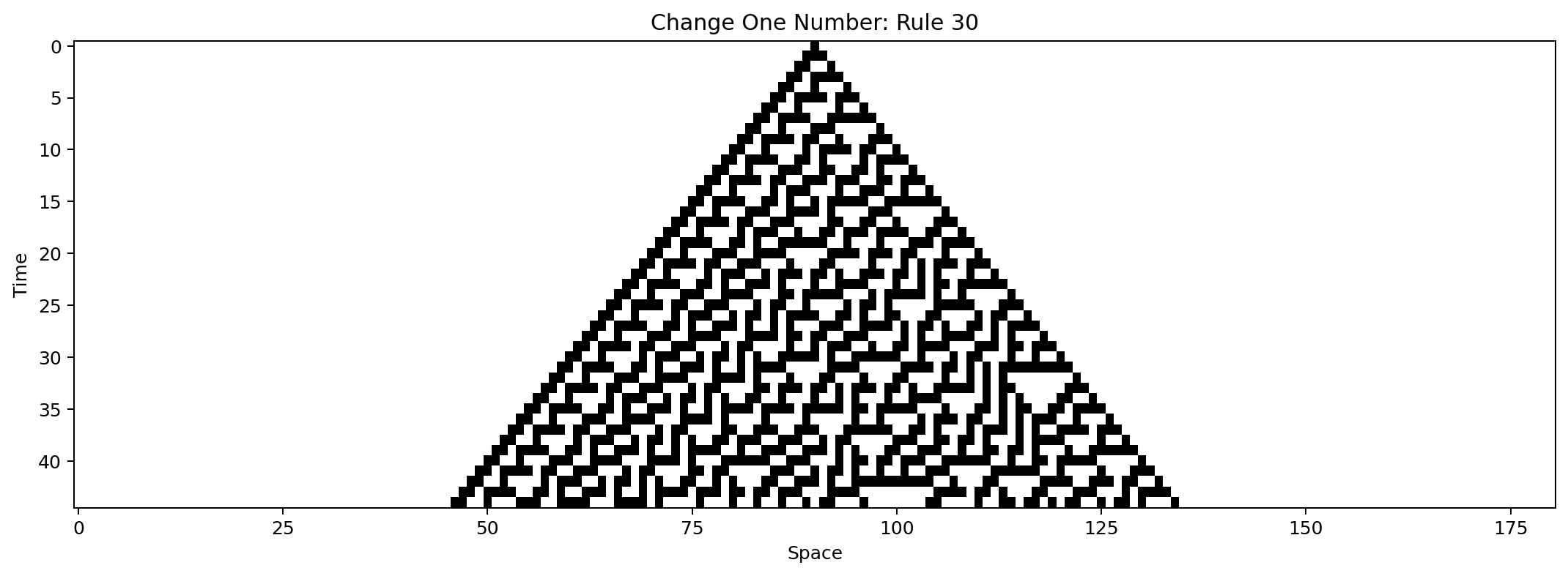
The result changes dramatically.

The machine is still tiny.

The mechanism is still entirely deterministic.

But the trajectory becomes much harder to dismiss as simple repetition.

That is where we go next.

We started with something creature-like.

We removed almost everything.

The mystery survived.

Next: The First Surprise.