The Space Between Models Has Holes: Mapping the AI Gap

🌌 Summary
What if the most valuable insights in AI evaluation aren’t in model agreements, but in systematic disagreements?
This post reveals that the “gap” between large and small reasoning models contains structured, measurable intelligence about how different architectures reason. We demonstrate how to transform model disagreements from a problem into a solution, using the space between models to make tiny networks behave more like their heavyweight counterparts.
We start by assembling a high-quality corpus (10k–50k conversation turns), score it with a local LLM to create targets, and train both HRM and Tiny models under identical conditions. Then we run fresh documents through both models, collecting not just final scores but rich auxiliary signals (uncertainty, consistency, OOD detection, etc.) and visualize what these signals reveal.
The core insight: use the “space around the score” to shrink the capability gap. We show how to standardize signals into Shared Core Metrics, create visual representation of each models knowledge, and apply lightweight calibration to make Tiny behave more like its big bro 👨👦 HRM where it matters.
What you’ll build with us:
- 🧠 Design, Implement train and use a new model the Tiny Recursive Model
- 🏋️♂️ Train HRM and Tiny on identical supervision from a local LLM
- 🌊 Use these trained models to score a large amount of similar data
- ⚖️ Extract, align, and standardize auxiliary diagnostics into a shared communication protocol
- 📸 Create visual analysis: score intensity images, frontier maps, and difference maps
- ✨ Discover information between or outside the model results, so in the area they are not talking about. This is the information in the
Gap. - 🔧 Implement practical calibration & routing that drive understanding of gap structure.
- 🤯 Use this same process on two unrelated Hugging Face models and find information there too.
Note: As the post developes it will get more technical. We have saved the difficult math code etc. for the appendices.
📃 Foundation Papers
Hierarchical Reasoning Model (HRM)
HRM: Hierarchical Reasoning Model
A hierarchical, multi-head reasoner with rich diagnostics and greater capacity.
We built and described this model here: Layers of thought: smarter reasoning with the Hierarchical Reasoning Model
Tiny Recursive Model (Tiny)
Tiny: Less is More: Recursive Reasoning with Tiny Networks
A compact, recursive scorer designed as a practical stand-in for HRM: faster, smaller, deployable.
As part of this post we will build describe and use this new model.
👁️ First Glimpse: The Gap Isn’t Empty
Before we dive into methodology, see what we mean by “structured disagreement”:
| Small vs Small | HRM vs Tiny (100) | HRM vs Tiny (500) | HRM vs Tiny (1000) |
|---|---|---|---|
 |
 |
 |
 |
| Small model disagreement | Emerging structure | Complex patterns | Stable features |
| Samples: 500 | Samples: 100 | Samples: 500 | Samples: 1000 |
| google/gemma-2-2b-it | HRM | HRM | HRM |
| HuggingFaceTB/SmolLM3-3B | Tiny | Tiny | Tiny |
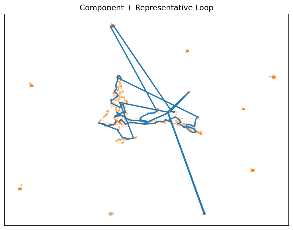
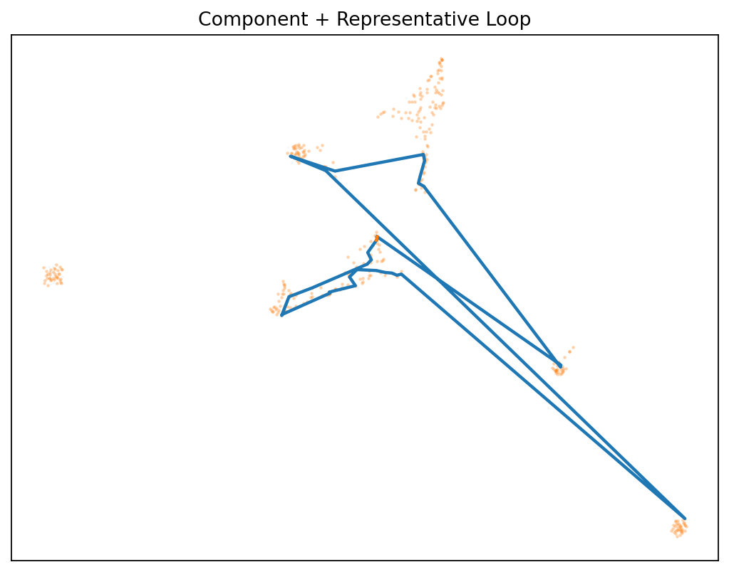
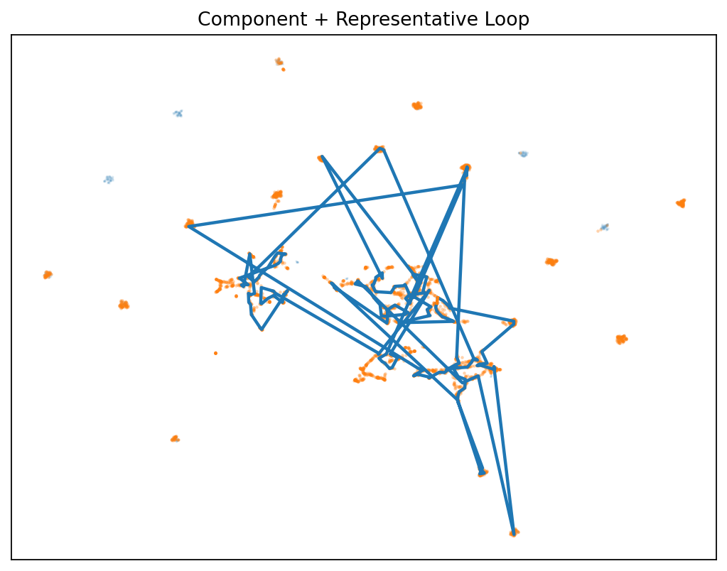
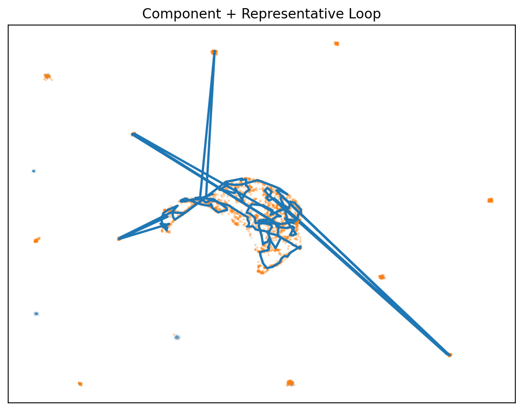
The discovery: Disagreement forms measurable structures that:
- 🌀 Persist as loops (H₁ homology) in the difference field
- 📈 Grow more complex with more samples
- 🔁 Replicate across architectures (local & Hugging Face)
- 🎯 Enable smarter routing between model capabilities
Once you can see the structure in disagreement space, you can route, calibrate, and train on the frontier.
📔 What Does It All Mean?
Same data. Same goal. Two minds. Different physics. We align them and visualize the layer in between.
Two models can reach similar answers while thinking completely differently. We take identical data and targets, run both HRM (heavyweight) and Tiny (lightweight), then ask: what lives in the space between them?
By aligning outputs and computing:
$$ \Delta = \text{HRM} - \text{Tiny} $$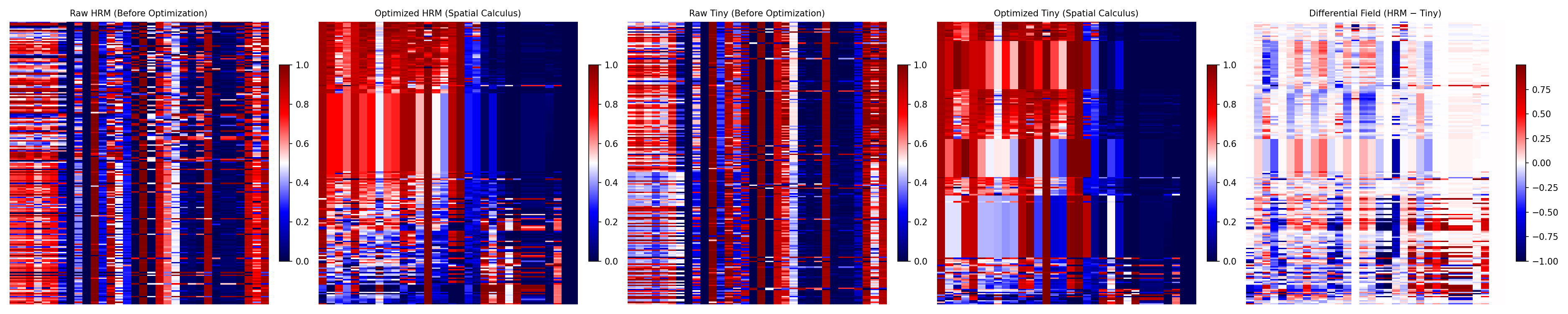 Vive la difference
- This shows the result of two AIs that both have been trained on th exact same information and are both trying to execute the same 1000 tasks. If they were perfect.
- If they were a perfect match the final image would be blank. This is what we mean when we say there is information in the Gap.
- The rest of this post will describe hwo we detected this information.
Ok so what?
The “between-space” becomes a visible field not featureless noise, but containing loops, clusters, and persistent structures that neither model shows alone.
The payoff: You’ll not only know what each model decides, but where each model can’t see and how to exploit those blind spots.
— Not
🔛 Preliminaries
These posts will help you understand some of the information in this post
| Post | Description | What it is used | Where Here |
|---|---|---|---|
| HRM | The post explains and implements the HRM model | Everything | This is the target model in our analysis |
| ZeroModel | The post explains ZeroModel | Used to generate VPM images adn do image analysis | The library is used to do the visual processing component |
| Phos | The post explains Phos a visual approach to AI | This post builds on that post | We extend the concepts in that post here |
👁️🗨️ What is Visual AI (short aside)
Instead of wading through logs, you see what the model is doing in real time.
| 🐞 Tiny (raw VPM with bug) | HRM (raw VPM) |
|---|---|
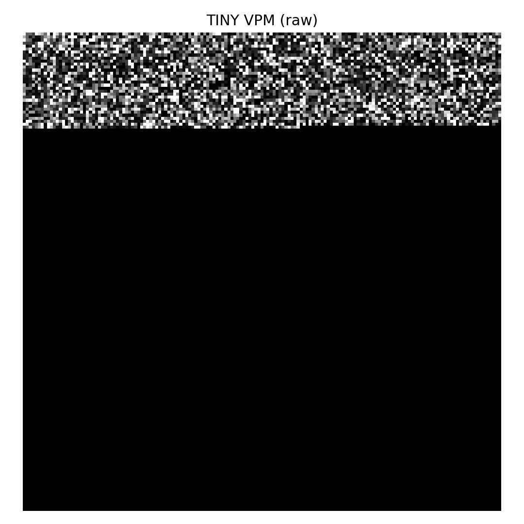 |
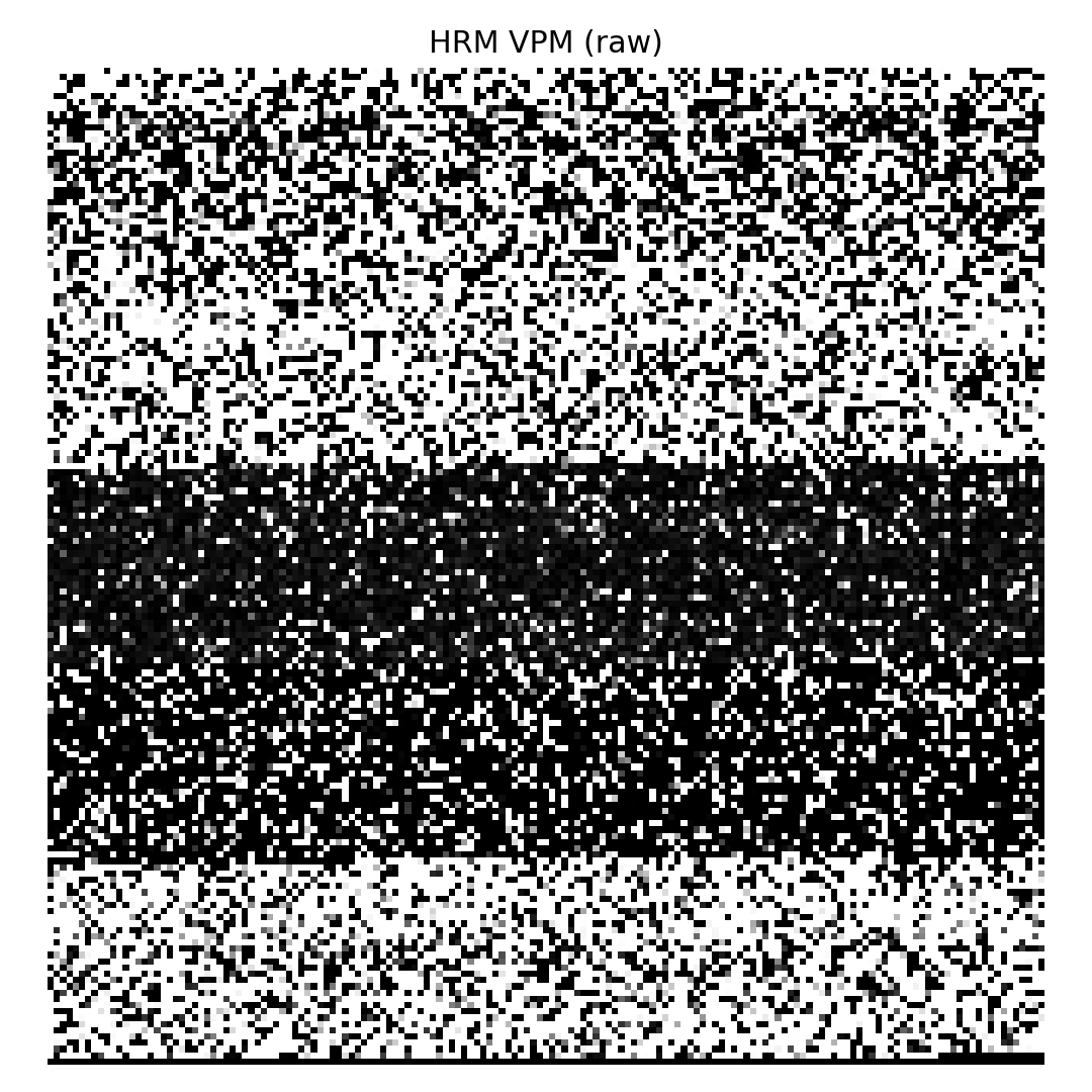 |
One glance = one diagnosis. A raw VPM tile is just turns × features reshaped to an image (rows ≈ turns, columns ≈ metric channels). In the Tiny pane, the single bright horizontal band means only one metric column was non-zero. In the HRM pane, texture appears across all features healthy.
What actually broke (Tiny): a heteroscedastic loss term (exp(-log_var)) blew up when log_var went very negative on non-reasoning dimensions. The precision term exploded, turning a sane loss (~6.38) into 221,118.81 within two epochs before NaN, silently zeroing those channels while the Reasoning channel (more stable) survived. The picture tells the story instantly no log spelunking required.
Plain English: one calculation went astronomically large, so everything else looked black by comparison.
Why Visual AI is ridiculously leverageful
They say a picture tells a thousand words. In our case, one tile encodes millions of signals:
- A 2400×2400 tile packs 5.76M pixel-level values.
- Each pixel corresponds to a concrete statistic (a score, residual, uncertainty, or latent).
- Your eye does instant change detection orders of magnitude more bandwidth than reading one scalar at a time.
So instead of comparing two numbers, you’re comparing two fields. The contrast between the Tiny and HRM images above makes the failure mode obvious at a glance. This is the core of Visual AI: turn numerical behavior into a visual artifact your brain can parse in milliseconds.
Craft notes (how we render these)
- We rasterize turns × features to a fixed canvas; each channel is min–max or robust-scaled per run for comparability.
- We keep a consistent dimension order (Reasoning, Knowledge, Clarity, Faithfulness, Coverage, …) so bands line up across runs.
- We ship both the raw arrays and the PNGs/GIFs pictures for humans, tensors for code.
If you remember one thing: a single glance can replace a million log lines and it will catch classes of failures (like exploding precision) that are easy to miss when you’re scrolling numbers.
✈️ Data Defines the Journey
Our dataset is our own conversation history with foundation models long, iterative chats aimed at building a self-improving AI so we know its character and quality, and that shaped every design choice we made (e.g., we didn’t have to lean hard on safety or faithfulness filters). Your journey may be different: if your conversations are noisier, safety-sensitive, or domain-specific, you’ll tune the pipeline differently (normalization, guardrails, faithfulness checks, caps). Key point: the dataset you start with determines the path you take mine yours for what matters to your goal, then adjust the knobs to fit your reality.
🧱 The Foundation: Multi-Dimensional Reasoning Scoring
Before we could compare reasoning models, we needed a consistent, structured way to evaluate reasoning itself. Traditional single-number scores collapse too much nuance good reasoning isn’t monolithic. It has facets.
So we defined five orthogonal dimensions that collectively capture what makes reasoning good:
| Dimension | What It Measures |
|---|---|
| Reasoning | Logical structure, multi-hop soundness, handling of assumptions and edge cases |
| Knowledge | Factual accuracy, specificity, and goal-advancing utility |
| Clarity | Organization, readability, scannability, and directness |
| Faithfulness | Consistency with context/goal, absence of hallucination |
| Coverage | Completeness across key facets implied by the question |
Note: we rejected some dimensions safety, faithfulness… because we were dealing data from foundation models and we know they would be very strong there.
- We wrote about dimensions here: Dimensions of Thought
- We wrote importing chat conversation history here: Episteme: Distilling Knowledge into AI
🌌 Why these five Dimensions?
We didn’t choose these arbitrarily. Through iterative analysis of high-quality vs. low-quality reasoning patterns, we identified these as the minimal set that:
- Covers distinct aspects of reasoning (minimal overlap)
- Is measurable with high inter-rater agreement
- Maps to observable improvements in downstream tasks
- Provides actionable feedback for refinement
Most importantly: these dimensions survive the “so what?” test. When we adjust a response to score higher in one dimension, human evaluators consistently rate it as better reasoning.
This common language is what makes the gap field visible without it, we’d be comparing apples to oranges.
🧭 The Scoring Engine prompts that make models think, not just rate
We don’t want numbers, we want reasoned numbers. The trick isn’t “ask for 1–5.” It’s forcing the model to analyze → decide → justify, in that order, for each dimension.
Our scoring engine wraps each dimension (Reasoning, Knowledge, Clarity, Faithfulness, Coverage) with a discipline loop:
- Narrow role → judge a single facet only
- Concrete criteria → what to reward & penalize
- Hard output contract → two lines: rationale + score
This converts vague ideas into stable, auditable signals.
The pattern (for one dimension: Knowledge)
SYSTEM:
You are a precise knowledge judge. You evaluate whether an assistant’s answer contains useful, true,
goal-advancing knowledge for the given user question. Be strict and concise.

CONVERSATION TITLE (goal):
{{ goal_text }}

USER QUESTION:
{{ user_text }}

ASSISTANT ANSWER:
{{ assistant_text }}

{% if context %}OK
OPTIONAL CONTEXT (may include prior turns, files, constraints):
{{ context }}
{% endif %}

{% if preferences %}
USER PREFERENCES (if any):
{% for p in preferences %}- {{ p }}
{% endfor %}
{% endif %}

INSTRUCTIONS:
1. Judge only the answer’s factual content and utility for the goal. Focus on specificity, correctness, and actionable details relevant to the question.
2. Reward: verifiably correct facts, precise terminology, concrete steps that advance the goal.
3. Penalize: hallucinations, outdated/wrong facts, irrelevant info, hedging without checks, missing key facts.
4. If there isn’t enough information to judge, treat as low score.

SCORING RUBRIC (whole numbers):
90–100: Accurate, specific, directly useful knowledge.
75–89: Mostly accurate and helpful; minor omissions.
60–74: Some value but notable uncertainty or gaps.
40–59: Weak; generic or risky to follow.
1–39: Poor; inaccurate/misleading.
0: Non-answer.

RETURN FORMAT (exactly two lines):
rationale: <brief reason, 1–3 sentences>
score: <0–100>
Why this works
- Narrow role prevents “dimension bleed” (e.g., docking Knowledge for writing style).
- Reward/Penalize lists anchor judgment in observable behaviors.
- Two-line contract forces think → commit → explain. Failures are obvious (bad format) and debuggable.
Five prompts, five lenses
We reuse the same skeleton, swapping the instruction block:
- Reasoning → structure, multi-hop soundness, assumptions/edge cases
- Knowledge → accuracy, specificity, goal-advancing utility
- Clarity → organization, scannability, directness
- Faithfulness → consistency with context/goal, no hallucination
- Coverage → completeness of key facets implied by the question
Together they produce a multi-dimensional profile of an answer. Adjust or add dimensions to match your domain (you could run 10–20 facets the same way).
Normalization (the “quiet” requirement)
Models emit 0–100. Normalize at ingestion:
score01 = round(score/100.0, 4)- Store both (
score,score01) plus the rationale - Keep dimension order fixed:
[reasoning, knowledge, clarity, faithfulness, coverage]
This prevents scale drift, enables cross-model comparison, and makes the Δ-field analysis meaningful.
Determinism & fairness knobs
- Temperature: 0–0.2 for scoring (stability > creativity).
- Identical context: pass the same goal/answer/context to every model.
- Token budget: trim to decision-critical snippets (but the same trim across models).
- Strict parser: reject outputs that violate the two-line format; log and retry once.
- Provenance: persist
model_name,model_version, prompt hash, and raw two lines.
Quick dimension blocks (drop-in text)
Use these inside the INSTRUCTIONS: section to retarget the same skeleton.
Reasoning
- Reward: explicit steps, correct chains, addressed edge cases, stated assumptions with checks.
- Penalize: leaps, circularity, contradictions, missing preconditions.
Clarity
- Reward: structure (lists, headings), concise phrasing, direct answers first, minimal fluff.
- Penalize: meandering, redundancy, buried ledes, jargon without necessity.
Faithfulness
- Reward: citations to the provided context, explicit limits, “cannot infer” when appropriate.
- Penalize: adding facts not in context, confident-but-wrong restatements.
Coverage
- Reward: touches all major facets implied by the goal, flags omissions explicitly.
- Penalize: single-facet answers to multi-facet questions, unacknowledged gaps.
Minimal parser (pseudo-Python)
def parse_two_line(output: str) -> tuple[str,int]:
    lines = [l.strip() for l in output.strip().splitlines() if l.strip()]
    assert len(lines) == 2 and lines[0].lower().startswith("rationale:") and lines[1].lower().startswith("score:")
    rationale = lines[0].split(":",1)[1].strip()
    score = int(lines[1].split(":",1)[1].strip())
    assert 0 <= score <= 100
    return rationale, score
On failure: record the raw text, one retry with a format-only fixer prompt, then mark as parser_error.
What this buys us downstream
- Auditable judgments (rationales) you can spot-check and learn from.
- Comparable numbers across models and runs (0–1 scale, fixed dimension order).
- Stronger Δ-signals: because each score was produced under the same disciplined reasoning routine.
Common pitfalls & quick fixes
- Drift into narrative → tighten “Be strict and concise”; cap rationale to ~300 chars.
- Dimension bleed → explicitly say “judge only this facet; ignore style/other facets.”
- Over-lenient 80–90s → add concrete failure modes in Penalize and examples of 60–74.
- Parser pain → keep “RETURN FORMAT (exactly two lines)” verbatim, fail fast on mismatch.
Bottom line: Scoring is not a number, it’s a procedure. Give the model a narrow job, unambiguous criteria, and a hard output contract. Do it per dimension, normalize, and log the rationale. That’s how you turn foundation models into consistent, high-signal judges and that’s what makes the gap field visible.
🔎 The Chat-Analyze Agent: how raw chats become labeled training data
This is the piece that turns conversations into numbers. It walks each user→assistant turn, applies our dimension-specific judges, parses the replies, and persists clean, normalized scores your downstream GAP pipeline can trust.
At a high level:
- Ingest turns from memory (or a provided batch).
- Load the right prompt for each dimension (Reasoning, Knowledge, Clarity, Faithfulness, Coverage).
- Call the judge LLM with
(goal, user, assistant[, context]). - Parse the strict 2-line response →
{rationale, score}. - Normalize score
0–100 → 0–1, record provenance, and persist. - Emit per-turn artifacts for dashboards (e.g., show Knowledge on the chat UI).
↩️ What it returns (example)
📊 knowledge_llm Dimension Scores conversation_turn:5962
+------------+-------+--------+----------------------------------------------+
| Dimension  | Score | Weight | Rationale (preview)                          |
+------------+-------+--------+----------------------------------------------+
| reasoning  | 95    | 1.0    | Coherent, technically accurate explanation… |
| knowledge  | 95    | 1.0    | Correct details of Epistemic HRM Scorer…    |
| clarity    | 98    | 1.0    | Exceptionally clear and well-structured…    |
| faithfulness| 95   | 1.0    | Matches code structure and purpose…          |
| coverage   | 95    | 1.0    | Addresses all key facets of the question…   |
| FINAL      | 95.6  |        | Weighted average                             |
+------------+-------+--------+----------------------------------------------+
👩💻 Minimal pseudocode (drop-in mental model)
def run_chat_analyze(context):
    # 0) Source turns
    turns = context.get("chats") or memory.chats.list_turns_with_texts(
        min_assistant_len=50, limit=cfg.limit, order_desc=False
    )

    analyzed = []
    for row in turns:
        # Skip if already scored (unless force_rescore)
        if row.get("ai_score") and not cfg.force_rescore:
            continue

        user_txt = row.get("user_text", "").strip()
        asst_txt = row.get("assistant_text", "").strip()
        if not user_txt or not asst_txt:
            continue

        # 1) Create/lookup a 'goal' from the user turn (provenance anchor)
        goal = memory.goals.get_or_create({
            "goal_text": user_txt,
            "description": "Created by ChatAnalyzeAgent",
            "pipeline_run_id": context.get("pipeline_run_id"),
            "meta": {"source": "chat_analyze_agent"},
        })

        per_dim = {}
        for dim in cfg.dimensions:  # ["reasoning","knowledge","clarity","faithfulness","coverage"]
            # 2) Load the dimension-specific prompt template
            prompt = prompt_loader.from_file(f"{dim}.txt", cfg, {**row, **context})
            # 3) Call LLM judge
            raw = prompt_service.run_prompt(prompt, {**row, **context})
            # 4) Parse strict output
            parsed = parse_judge(raw)  # -> {"rationale": str, "score": int 0..100}
            score01 = parsed["score"] / 100.0

            per_dim[dim] = ScoreResult(
                dimension=dim,
                score=score01,
                source="knowledge_llm",
                rationale=parsed["rationale"],
                attributes={"raw_response": raw, "score100": parsed["score"]},
            )

            # Optional: write Knowledge score back to chat for GUI
            if dim == "knowledge":
                memory.chats.set_turn_ai_eval(
                    turn_id=row["id"], score=parsed["score"], rationale=parsed["rationale"]
                )

        # 5) Persist as one bundle (with provenance)
        scoring.save_bundle(
            bundle=ScoreBundle(results=per_dim),
            scorable=Scorable(id=row["assistant_message_id"], text=asst_txt, target_type=CONVERSATION_TURN),
            context={**context, "goal": goal.to_dict()},
            cfg=cfg, agent_name="chat_analyze_agent", scorer_name="knowledge_llm", source="knowledge_llm",
            model_name="llm",
        )

        analyzed.append({
            "turn_id": row["assistant_message_id"],
            "score": per_dim["knowledge"].attributes["score100"],  # convenience for UI
            "rationale": per_dim["knowledge"].rationale,
        })

    return {**context, "analyzed_turns": analyzed}
👖 How the prompt loader fits
-
Template per dimension (
reasoning.txt,knowledge.txt, …) contains:- the system role, the input slots (
goal_text,user_text,assistant_text,context,preferences), and - the strict two-line return format.
- the system role, the input slots (
-
The loader simply renders the right template with the turn payload, so judges see identical structure run-to-run.
💰 Implementation tips
- Normalization: always divide the 0–100 by 100 before any analytics (GAP, topology, viz).
- Strict parsing: enforce the 2-line contract; fail closed (raise
ParseError) and log the raw response. - Idempotency: use
force_rescoreto override; otherwise skip already-scored turns. - Provenance: store
turn_id,assistant_message_id,goal_id,scorer_name/version,pipeline_run_id. - Batching & retries: add small jittered retries for judge calls; backoff on rate limits.
- Guardrails: drop turns with missing text, or those exceeding your token/char budget for the judges.
With this agent in place, you get a clean, reproducible labeled corpus that reflects how well answers perform along our five dimensions ready for GAP analysis, model training, and Visual-AI diagnostics.
🏗️ Model Building
(HRM + Tiny) and a shared protocol so they can actually be compared
This section is about how we build the models and, more importantly, how we make their outputs commensurable.
🤷 What we’re building
-
HRM (re-intro) We reuse the HRM architecture from our earlier post (linking there for details), and treat it as our high-fidelity reference scorer.
-
Tiny (from scratch) We implement the Tiny scorer end-to-end: model → trainer → scorer. Tiny is intentionally small and fast so we can iterate quickly, ship to edge boxes, and stress the tooling.
-
A shared protocol of attributes We extend both HRM and Tiny to report the same, standardized set of diagnostic attributes alongside their per-dimension scores. This protocol is what lets us align two very different systems without forcing one to imitate the other’s internals.
Why this matters: direct “metric mapping” (e.g., “uncertainty ≈ logvar here, ≈ entropy there”) looked neat on paper but failed in practice different models compute/represent those notions differently. Our fix is to define the outputs we want (common semantics) and make each model emit them in a canonical format.
🤝 The shared protocol SCM
We call the protocol SCM (Shared Canonical Metrics). Each model must produce:
-
Per-dimension, normalized scores (0–1)
scm.reasoning.score01,scm.knowledge.score01,scm.clarity.score01,scm.faithfulness.score01,scm.coverage.score01 -
Aggregate
scm.aggregate01simple average over the five dimensions (or a documented weighted average) -
Process diagnostics (model-agnostic definitions)
scm.uncertainty01normalized predictive uncertainty (e.g., entropy normalized by log-vocab)scm.ood_hat01out-of-distribution proxy (e.g., PPL normalized to a band)scm.consistency01internal consistency proxy (e.g., sigmoid of mean logprob blended with 1−uncertainty)scm.length_norm01normalized token length to discourage score inflation by verbosityscm.temp01temperature proxy (we mirror uncertainty here so downstream plots have a stable axis)scm.agree_hat01agreement proxy (e.g., logistic transform of mean logprob)
These are not the models’ native losses or hidden states; they’re standardized readouts. Each model computes its own way to populate them, but the semantics and scale are fixed so Δ-analysis (A−B) is well-posed.
🎨 What the section will cover
-
HRM recap (short, with link): objectives, inductive biases, where it shines.
-
Tiny build (full):
- architecture choices and why (small, stable, debuggable)
- training loop (datasets from Chat-Analyze Agent, loss design, stability guardrails)
- evaluation harness and scorer interface
-
Protocol integration (both models): how we compute each SCM field, normalization details, and test vectors to verify parity.
-
Why this protocol beats ad-hoc mappings: examples where naive “map X→Y” failed, and how SCM gives clean apples-to-apples deltas.
Bottom line: We’re not trying to make Tiny “be HRM.” We’re making both models speak the same measurement language. Once they emit SCM, we can compare, visualize, and reason about the gap field with confidence.
👑 The Hierarchical Reasoning Model: A Deep Reasoning Engine
While Tiny is our fast inner loop, HRM is the deep, high-fidelity judge we lean on when we need comprehensive reasoning diagnostics.I
💖 We have seen HRM before
| What | Description |
|---|---|
| 📚 Layers of Thought | Blog post where we go over how we integrated HRM into Stephanie |
| 🧑🎤 Model | Model Implementation Source Code |
| 🏋️♀️ Trainer | Class Used to train the HRM model |
| ⚽ Scorer | The scoring implementation for the HRM class |
👯 The Dual-Recurrent Architecture
HRM’s power comes from its two coupled recurrent networks operating at different temporal scales:
# Hierarchical recurrent modules
self.l_module = RecurrentBlock(2 * self.h_dim, self.l_dim, name="LModule")
self.h_module = RecurrentBlock(self.l_dim + self.h_dim, self.h_dim, name="HModule")All right can you please address this
This creates a processing hierarchy where:
- Low-level (L) module performs fine-grained analysis (4 steps per cycle)
- High-level (H) module integrates information across longer time horizons (1 step per cycle)
During evaluation, HRM executes this hierarchical processing across multiple cycles:
for cycle in range(self.n_cycles):
    # Low-level fine-grained processing (T steps)
    for step in range(self.t_steps):
        l_input = torch.cat([x_tilde, zH], dim=-1)
        zL = self.l_module(zL, l_input)

    # High-level abstract update (1 step per cycle)
    h_input = torch.cat([zL, zH], dim=-1)
    zH = self.h_module(zH, h_input)
This dual-frequency approach allows HRM to capture both detailed reasoning steps and higher-level patterns making it particularly effective for complex, multi-hop reasoning tasks.
🟰 Multi-Dimensional Quality Assessment
Unlike simple scoring systems, HRM generates a rich diagnostic surface across five key reasoning dimensions we’ve defined:
| Dimension | What HRM Measures |
|---|---|
| Reasoning | Logical structure, multi-hop soundness, handling of assumptions |
| Knowledge | Factual accuracy and specificity |
| Clarity | Organization, readability, and directness |
| Faithfulness | Consistency with context/goal, absence of hallucination |
| Coverage | Completeness across key facets |
For each dimension, HRM doesn’t just produce a score it generates a comprehensive diagnostic profile:
# Core diagnostic heads
self.score_head       = nn.Linear(self.h_dim, 1)  # quality logits
self.logvar_head      = nn.Linear(self.h_dim, 1)  # aleatoric uncertainty
self.aux3_head        = nn.Linear(self.h_dim, 3)  # bad/medium/good aux
self.disagree_head    = nn.Linear(self.h_dim, 1)  # predicted disagreement
self.consistency_head = nn.Linear(self.h_dim, 1)  # robustness proxy
self.ood_head         = nn.Linear(self.h_dim, 1)  # OOD proxy
# (optionally) temperature / calibration head for score scaling
This produces not just a score (0-100), but also:
uncertainty: How confident is this score?consistency_hat: How robust is the score to input variations?ood_hat: Is this response out-of-distribution?jacobian_fd: How sensitive is the score to tiny input changes?
🔗 How HRM populates the shared protocol (SCM)
To compare HRM with Tiny, both speak SCM (Shared Canonical Metrics). HRM fills:
| SCM field | How HRM computes it (intuition) |
|---|---|
scm.<dim>.score01 |
sigmoid(calibrated(score_head)) per dimension → [0,1] |
scm.aggregate01 |
mean of the five score01 (or documented weighted mean) |
scm.uncertainty01 |
normalized entropy / uncertainty from logvar_head or logits |
scm.consistency01 |
blend of sigmoid(mean_logprob) and 1−uncertainty01 |
scm.ood_hat01 |
normalized proxy from ood_head or PPL banding |
scm.length_norm01 |
token-length min–max clamp to [0,1] |
scm.temp01 |
mirrors uncertainty (stable axis for visuals) |
scm.agree_hat01 |
agreement proxy from score logit / mean logprob |
Scale discipline: HRM produces score01 ∈ [0,1] for SCM; UI “/100” views are derived by
round(100*score01)for readability.
🏅 Why HRM Matters for This Comparison
HRM serves as our gold-standard reasoning evaluator the deep, comprehensive system against which we measure Tiny’s lightweight approach. The key insight is that HRM and Tiny aren’t competing systems they’re complementary layers in Stephanie’s cognitive architecture.
HRM is designed for:
- Deep multi-step reasoning validation
- Complex plan analysis
- Comprehensive quality assessment
While powerful, HRM’s strength comes with computational cost making it less suitable for:
- Real-time refinement
- Edge deployment
- Continuous self-correction
This is precisely where Tiny enters the picture, not to replace HRM but to amplify it with a fast, recursive inner loop that handles the “polishing” work before responses reach users or trigger deeper HRM analysis.
By understanding HRM’s deep reasoning capabilities, we can better appreciate how Tiny’s lightweight approach captures the essential patterns that make reasoning good without the computational overhead.
❗ The Disagree Head what it is (and why it matters)
We reference a “disagree head” in diagrams; here’s the explicit meaning:
-
What it predicts: A proxy for where Tiny and HRM are likely to diverge on quality for the same input.
-
How it trains: Using past pairs where we observed an absolute delta (e.g.,
|score01_hrm − score01_tiny|) above a margin; we treat that as a target disagreement event. The head learns a logit → probability that such a divergence will occur again on similar patterns. -
How we use it:
- If
sigmoid(disagree_head)is high, route the case to HRM (don’t trust Tiny alone). - If low, Tiny’s light-weight signal is usually safe, keeping latency down.
- If
SCM mapping: scm.agree_hat01 = 1 − sigmoid(disagree_head) gives a standardized agreement confidence (1 = likely to agree).
Intuition: the head isn’t “reading Tiny’s mind”; it learns situations (content/process patterns in
zH) where Tiny historically missed nuance HRM caught (e.g., multi-hop edge cases, subtle factual grounding).
🧯 Stability guardrails (what we fixed)
Earlier we hit heteroscedastic loss blow-ups (exp(-log_var)) on non-reasoning heads. Fixes:
- Softplus floor on
log_var(prevents extreme negatives), - Gradient clipping across heads,
- Per-head loss caps to stabilize batches.
Result: all five dimensions train cleanly; numbers stay finite.
    graph TD
    %% Title and Input Section
    A[🎯 HRM Hierarchical Reasoning Model<br/>Multi-Head Architecture] --> B[📥 Input Layer]

    B --> C[🔮 Input Projector<br/>x → x̃]

    %% Hierarchical Core Processing
    C --> D{🔄 Hierarchical Core<br/>Dual Recurrent Processing}

    D --> E[🐢 Low-Level Module L<br/>Fine-grained Analysis<br/>T steps per cycle]
    D --> F[🐇 High-Level Module H<br/>Abstract Reasoning<br/>1 step per cycle]

    E --> G[🔄 State Feedback Loop]
    F --> G
    G --> D

    %% Final States
    D --> H[💎 Final States<br/>zL_final + zH_final]

    %% Primary Scoring Pathway
    H --> I[🌡️ Temperature Head<br/>τ calibration]
    H --> J[⭐ Score Head<br/>Quality logits]

    I --> K[🎯 Primary Score<br/>score01 ∈ 0,1<br/>Temperature calibrated]
    J --> K

    %% Uncertainty & Confidence Heads
    H --> L[📊 LogVar Head<br/>Aleatoric uncertainty]
    H --> M[🔢 Aux3 Head<br/>Bad/Medium/Good]

    L --> N[✅ Certainty01<br/>Uncertainty measure]
    M --> O[📶 Entropy Aux<br/>Confidence score]

    %% Agreement & Robustness Heads
    H --> P[⚔️ Disagree Head<br/>HRM-Tiny disagreement]
    H --> Q[🛡️ Consistency Head<br/>Robustness prediction]

    P --> R[🔄 Disagree Hat<br/>Predicted disagreement]
    Q --> S[🎯 Consistency Hat<br/>Robustness score]

    %% Specialized Diagnostic Heads
    H --> T[🚫 OOD Head<br/>Out-of-distribution]
    H --> U[🔁 Recon Head<br/>Input reconstruction]
    H --> V[📏 Jacobian FD<br/>Sensitivity analysis]

    T --> W[🎯 OOD Hat<br/>Anomaly detection]
    U --> X[📐 Recon Sim<br/>Comprehension quality]
    V --> Y[📊 Jacobian FD<br/>Input sensitivity]

    %% Evidence Accumulation
    H --> Z[🛑 Halt Signal<br/>Evidence accumulation]
    Z --> AA[🎲 Halt Prob<br/>Pseudo-halting]

    %% Styling and Grouping
    classDef input fill:#e3f2fd,stroke:#1976d2,stroke-width:2px,color:#0d47a1
    classDef core fill:#fff3e0,stroke:#e65100,stroke-width:3px
    classDef primary fill:#e8f5e8,stroke:#2e7d32,stroke-width:3px
    classDef uncertainty fill:#fce4ec,stroke:#c2185b,stroke-width:2px
    classDef agreement fill:#e3f2fd,stroke:#1565c0,stroke-width:2px
    classDef diagnostic fill:#f3e5f5,stroke:#7b1fa2,stroke-width:2px
    classDef evidence fill:#fff8e1,stroke:#ff8f00,stroke-width:2px

    class A,B,C input
    class D,E,F,G core
    class I,J,K primary
    class L,M,N,O uncertainty
    class P,Q,R,S agreement
    class T,U,V,W,X,Y diagnostic
    class Z,AA evidence

    %% Legend
    subgraph Legend[📖 Legend - Head Types]
        L1[🟩 Primary Scoring] --> L2[🟥 Uncertainty & Confidence]
        L2 --> L3[🟦 Agreement & Robustness]
        L3 --> L4[🟪 Specialized Diagnostics]
        L4 --> L5[🟨 Evidence Accumulation]
    end
🎯 Why Tiny? And How the Gap Emerged
We didn’t set out to “prove a theory.” We saw the Tiny paper on Hugging Face, loved the idea of a compact DNN that sits between heavyweight models and applications, and knew instantly it fit Stephanie’s architecture. We implemented it because it was useful fast, small, and easy to deploy where HRM is too heavy. That was the whole plan.
Then something clicked.
🧮 From “stacking signals” to “subtracting signals”
Our first idea was straightforward: append Tiny’s diagnostics to HRM’s output to get more information per turn. Extra signal, same data. Great.
But while wiring that up, we asked a different question: What if we subtract instead of append?
If two evaluators look at the same conversation and we align their outputs into the same schema (SCM), then the difference between them should reveal something real:
$$[ \Delta(h) = \text{HRM}(h) - \text{Tiny}(h) ]$$We didn’t know there was anything meaningful in Δ. We suspected there had to be call it a Holmes-style deduction: remove everything both models agree on; what remains is the interesting part.
✔️ The moment of confirmation: Betti numbers
We ran persistent homology on Δ and the Betti-1 counts spiked consistently. The topology of the gap wasn’t noise; it had structure (loops) that stayed under resampling. That was the “oh wow” moment. We still can’t name the exact cause of every loop but like electricity, you don’t have to fully explain it to measure, improve, and use it.
🎯 What we’re actually after
Our north star is self-improving AI especially learning from hallucinations rather than just suppressing them. Tiny gave us a new lens. HRM gave us depth. Δ gave us a map of where evaluators diverge in systematic ways. That map is where:
- escalation policies get smart (when Tiny says “I’m uncertain/OOD/disagree,” hand off to HRM),
- training data gets targeted (hotspots on the Δ field),
- and future posts (next: “learning from hallucination”) get their raw material.
👍 Why Tiny was the right instrument (even before Δ)
- It runs in milliseconds and can live at the edge or in inner loops.
- It produces diagnostics (uncertainty, OOD, sensitivity, agreement) we can align with HRM via SCM.
- It gave us a second, independently trained viewpoint on the same data exactly what you need to make Δ meaningful.
📑 How to replicate the pivot (in three steps)
- Align: score the same conversations with two evaluators (we used HRM and Tiny) and write both to SCM (0–1, same keys/order).
- Subtract: compute (\Delta = A - B) per turn (dimension-wise).
- Probe: run PH (Vietoris–Rips), examine Betti-1 persistence; cluster Δ-hotspots for inspection and distillation.
We started by stacking, but the real insight came from subtracting. Tiny didn’t just add signal it revealed where signal differs, and that’s the raw ore we can mine.
❌ What this isn’t
- It’s not a claim that Tiny “beats” HRM. They’re complementary.
- It’s not a proof of a specific cognitive mechanism. It’s a measurement pipeline that repeatedly shows structure where naïvely you’d expect noise.
🔜 What comes next
- We’ll use Δ-hotspots to drive targeted training and hallucination learning (next post).
- We’ll keep strengthening SCM so any new scorer can be dropped in and compared locally or on HF.
That’s the honest path: we implemented Tiny because it was obviously useful. The gap emerged when we switched from adding to subtracting, and the topology told us we’d found something worth pursuing.
🌀 The Tiny Recursion Model and our instrumented Tiny+
Tiny is a small, recursive evaluator that operates directly in embedding space. It produces a fast, multi-signal judgment about a response (quality, uncertainty, OOD, sensitivity, etc.). Tiny+ is our instrumented version of Tiny: same core, but wired into our SCM (Shared Canonical Metrics) protocol and extended with a few probes that make Tiny and HRM directly comparable for Δ-field analysis.
One-liner: Tiny is a general-purpose, parameter-efficient evaluator; Tiny+ is how we adapted it for Stephanie’s gap work.
🤔 Why Tiny exists (beyond our stack)
Tiny stands on its own. It’s useful wherever you need cheap, consistent signals about model outputs:
- Edge / low-latency scoring on CPU
- Cost-aware routing (decide when to call a heavier judge/model)
- Eval/A-B pipelines as a stable, repeatable rater
- Drift & health monitoring (OOD + sensitivity) on production traffic
- Retrieval/reranking (blend quality, uncertainty, and stability)
- Teacher–assistant distillation (soft targets + confidence)
We use Tiny+ inside Stephanie to align with HRM and visualize Δ, but the architecture is system-agnostic.
🏢 Architecture at a glance
    graph TD
    %% Title and Input Section
    A["🤖 Tiny Recursion Model (Tiny+)<br/>Multi-Head Recursive Architecture"All right] --> B[🎯 Triple Input Layer]
    B --> C[📥 Goal Embedding x]
    B --> D[💬 Response Embedding y]
    B --> E[🌀 Initial Latent z]
    %% Recursive Fusion Core
    C --> F{🔄 Recursive Fusion Core<br/>N Recursion Steps}
    D --> F
    E --> F
    F --> G["🔗 State Fusion<br/>x ⊕ y ⊕ z → z_next"]
    G --> H[🏗️ Core Processing<br/>MLP/Attention Blocks]
    H --> I[🛑 Halting Signal<br/>Step-wise accumulation]
    I --> J[⚖️ Residual Update<br/>z = z + step_scale × z_next]
    J --> F
    %% SAE Bottleneck
    F --> K[💎 Final State z_final]
    K --> L[🧠 Sparse Autoencoder<br/>SAE Bottleneck]
    L --> M[🔍 Concept Codes c<br/>Sparse representation]
    L --> N[🎛️ Head State z_head<br/>SAE reconstruction]
    %% Primary Scoring Pathway
    N --> O[🌡️ Temperature Head<br/>τ calibration]
    N --> P[⭐ Score Head<br/>Quality logits]
    O --> Q["🎯 Primary Score<br/>s ∈ 0,1<br/>Temperature calibrated"]
    P --> Q
    %% Uncertainty & Confidence Heads
    N --> R[📊 LogVar Head<br/>Aleatoric uncertainty]
    N --> S[🔢 Aux3 Head<br/>Bad/Medium/Good]
    R --> T[✅ Certainty01<br/>Uncertainty measure]
    S --> U[📶 Entropy Aux<br/>Confidence score]
    %% Agreement & Disagreement Heads
    N --> V[⚔️ Disagree Head<br/>HRM-Tiny disagreement]
    N --> W[🤝 Agree Head<br/>Cross-model agreement]
    V --> X[🔄 Disagree Hat<br/>Predicted disagreement]
    W --> Y[🎯 Agree01<br/>Agreement probability]
    %% Robustness & Reconstruction Heads
    N --> Z[🛡️ Consistency Head<br/>Robustness prediction]
    N --> AA[🔁 Recon Head<br/>Response reconstruction]
    Z --> BB[🎯 Consistency Hat<br/>Robustness score]
    AA --> CC[📐 Recon Sim<br/>Reconstruction quality]
    %% Specialized Diagnostic Heads
    N --> DD[🚫 OOD Head<br/>Out-of-distribution]
    N --> EE[📏 Jacobian FD<br/>Sensitivity analysis]
    N --> FF[📏 Causal Sens Head<br/>Perturbation sensitivity]
    DD --> GG[🎯 OOD Hat<br/>Anomaly detection]
    EE --> HH[📊 Jacobian FD<br/>Input sensitivity]
    FF --> II[🎯 Sens01<br/>Sensitivity measure]
    %% Length Normalization
    JJ[📏 Sequence Length] --> KK[⚖️ Length Effect<br/>Normalization]
    KK --> LL[📐 Len Effect<br/>Length adjustment]
    %% Legacy Outputs
    N --> MM[📚 Classifier Head<br/>Legacy vocab logits]
    I --> NN[🛑 Halt Logits<br/>Step accumulation]
    %% Styling and Grouping
    classDef input fill:#e1f5fe,stroke:#01579b,stroke-width:2px
    classDef core fill:#fff3e0,stroke:#e65100,stroke-width:3px
    classDef sae fill:#e8f5e8,stroke:#2e7d32,stroke-width:3px
    classDef primary fill:#e8f5e8,stroke:#2e7d32,stroke-width:3px
    classDef uncertainty fill:#fce4ec,stroke:#c2185b,stroke-width:2px
    classDef agreement fill:#e3f2fd,stroke:#1565c0,stroke-width:2px
    classDef robustness fill:#fff3e0,stroke:#ff6f00,stroke-width:2px
    classDef diagnostic fill:#f3e5f5,stroke:#7b1fa2,stroke-width:2px
    classDef legacy fill:#f5f5f5,stroke:#616161,stroke-width:2px
    class A,B,C,D,E input
    class F,G,H,I,J core
    class L,M,N sae
    class O,P,Q primary
    class R,S,T,U uncertainty
    class V,W,X,Y agreement
    class Z,AA,BB,CC robustness
    class DD,EE,FF,GG,HH,II diagnostic
    class JJ,KK,LL,MM,NN legacy

    %% Legend
    subgraph Legend[📖 Legend - Head Types]
        L1[🟩 Primary Scoring] --> L2[🟥 Uncertainty & Confidence]
        L2 --> L3[🟦 Agreement & Disagreement]
        L3 --> L4[🟧 Robustness & Reconstruction]
        L4 --> L5[🟪 Specialized Diagnostics]
        L5 --> L6[⬜ Legacy & Utilities]
    end
Inputs
x: goal/condition embedding[B, D]y: response embedding[B, D]z: latent state (init zeros)[B, D]
Core loop (n recursions)
- Fuse
[x, y, z] → z'viaLinear + tanh - Process with a compact stack (MLP or MHA blocks)
- Update
z ← z + step_scale * z'(residual step) - Track halting logits (max over steps)
Bottleneck
- SAE (Sparse Autoencoder) over
z_final→ sparse codesc - Reconstruct to
z_headfor all output heads (acts like a concept layer)
Heads (multi-task)
- Score, (log) uncertainty, OOD, consistency/robustness, temperature proxy
- Agreement/disagreement (for parity), finite-difference sensitivity
- Reconstruction similarity (for concept fidelity)
# Core residual block (MLP) or attention variant
class TinyBlock(nn.Module): ...
class TinyBlockAttn(nn.Module): ...

# Recursion (sketch)
fused   = torch.cat([x, y, z], -1)
z_next  = torch.tanh(W @ fused) → core blocks
z       = z + step_scale * z_next  # repeat n times

# SAE bottleneck → heads
c       = SAE_enc(z_final)               # sparse codes
z_head  = z_final + SAE_dec(c)           # head input
# Heads read from z_head (score/logvar/ood/consistency/etc.)
🚧 Numerical safety & calibration (baked in)
- Aleatoric clamp:
log_var ∈ [−5, 5](prevents precision explosions) - Temperature calibration:
tau = 0.5 + 0.5 * softplus(·),score01 = σ(score_logit / tau)(stable, calibrated) - Sensitivity proxy: finite-difference on a normalized perturbation, clipped
- Length proxy:
length_norm01 = (tanh(len/L)+1)/2avoids “long = always bad”
These keep Tiny stable across 4k–8k token regimes and varied difficulty.
🗣️ Heads → SCM (so Tiny and HRM speak the same language)
Tiny+ writes aligned telemetry into SCM, so Δ = HRM − Tiny is meaningful:
| SCM key | Tiny(+ ) source (range) | Meaning |
|---|---|---|
scm.<dim>.score01 |
σ(score_logit / tau) (0..1) |
Per-dimension quality (copy to each dim you evaluate) |
scm.aggregate01 |
mean of per-dim score01 |
Overall quality |
scm.uncertainty01 |
1 − σ(−log_var) (0..1) |
Aleatoric uncertainty |
scm.consistency01 |
σ(consistency_logit) (0..1) |
Robustness to masking/perturbations |
scm.ood_hat01 |
σ(ood_logit) (0..1) |
Out-of-distribution proxy |
scm.temp01 |
σ(tau_raw) (0..1) |
Temperature/entropy proxy (alignment key) |
scm.jacobian_fd |
clipped FD sensitivity (0..1) | Score sensitivity to small input changes |
scm.length_norm01 |
bounded length proxy (0..1) | Normalized response length effect |
scm.agree_hat01 |
1 − σ(disagree_logit) (0..1) |
Predicted agreement with a reference judge (HRM in our stack) |
scm.recon_sim01 |
cosine(ŷ, y) mapped to (0..1) | Concept fidelity via SAE reconstruction |
Bonus: expose
concept_sparsityfor Visual-AI panes (instant concept heat).
➕ Why Tiny is more than “HRM but small”
Different objective and operating point:
- HRM does deep semantic validation; Tiny diagnoses meta-signals agreement, uncertainty, OOD, sensitivity that tell you when light-weight judgment is safe vs. when to escalate.
- Tiny runs on fixed embeddings with compact recursion; it’s cheap enough for the inner loop and edge.
The combination builds a cost-aware evaluator: Tiny handles the confident in-distribution mass; it forwards the risky tail to HRM.
🗳️ Practical decision patterns
- High
ood_hat01+ highagree_hat01→ unusual, but HRM likely agrees → ok to serve. - High
ood_hat01+ lowagree_hat01→ unusual and likely disagreement → escalate. - High
jacobian_fd+ lowconsistency01→ fragile judgment → escalate. - High
uncertainty01+ lowtemp01→ uncertain & poorly calibrated → caution.
👀 SAE bottleneck: making the unseen visible
The SAE forces a sparse concept code. Two wins:
- Interpretability:
concept_sparsityandrecon_sim01show when Tiny relies on a small, stable set of “ideas” vs. diffuse noise. - Transfer: concepts that remain predictive across datasets tend to align with durable reasoning patterns great anchors for Δ-attribution.
👶 Minimal “generic” API (no Stephanie dependencies)
# Example usage outside Stephanie
x  = embed(goal_text)                 # [B, D]
y  = embed(response_text)             # [B, D]
z0 = torch.zeros_like(x)

_, _, _, aux = tiny(x, y, z0, seq_len=len_tokens(response_text), return_aux=True)

result = {
  "score01":        float(aux["score"].mean()),
  "uncertainty01":  float(aux["uncertainty01"].mean()),
  "ood01":          float(aux["ood_hat01"].mean()),
  "consistency01":  float(aux["consistency_hat"].mean()),
  "sensitivity01":  float(aux["jacobian_fd"].mean()),
  "length_norm01":  float(aux["length_norm01"].mean()),
}
# Use for routing, monitoring, ranking, or eval.
If you adopt SCM, just map these to your preferred keys (we use scm.* for cross-model alignment).
🎲 Design choices that mattered
- Clamp
log_varand deriveuncertainty01 = 1 − σ(−log_var)(monotone, stable, interpretable). - Use
temp01 = σ(tau_raw)for alignment; keeptaufor calibration math. - Sensitivity proxy: normalize perturbations and clip
jacobian_fd. - SAE α ≈ 0.05: enough sparsity pressure without crushing expressivity.
- Length proxy: bounded
tanh(len/L)mapped to[0,1]avoids pathological length effects.
🌀 Tiny+ in Stephanie (what’s different)
- SCM wiring so Tiny and HRM align 1:1
- Agreement/disagreement head tuned for HRM parity and Δ analysis
- Visual-AI first: outputs designed to render as “turns × features” images for instant diagnosis
This is how we compute Δ = HRM − Tiny per turn/dimension and then study its topology (e.g., persistent loops).
📅 What’s next in this post
Up next is the full Tiny source (model), followed by the trainer and the scorer wrapper. If you just want the gist, the sections above are enough to implement a compatible Tiny. If you enjoy digging into details: the code that follows is production-hardened, numerically safe, and instrumented for Δ-field work.
Tiny Recursion Model: View full source
# stephanie/scoring/model/tiny_recursion.py
"""
Tiny Recursion Model (Tiny+) - Parameter-Efficient Recursive Neural Architecture

This module implements a compact, recursive neural network for multi-task evaluation
of AI model responses. The architecture combines recursive state updates with
multi-head output predictions, enabling efficient quality assessment across
multiple dimensions from embedding inputs.

Key Innovations:
- Recursive latent state updates with halting mechanisms
- Sparse Autoencoder (SAE) bottleneck for interpretable concepts
- Multi-head prediction for comprehensive quality assessment
- Heteroscedastic uncertainty estimation
- In-graph consistency regularization

Architecture Overview:
1. Recursive fusion of goal (x), response (y), and latent (z) states
2. Core processing blocks (attention or MLP-based)
3. SAE bottleneck for sparse concept representation
4. Multi-head prediction for scores, uncertainty, and auxiliary tasks

"""

from __future__ import annotations

from typing import Any, Dict, Optional, Tuple

import torch
import torch.nn as nn
import torch.nn.functional as F

# ---------------------------
# Core Building Blocks
# ---------------------------

class TinyBlock(nn.Module):
    """
    Basic residual block: LayerNorm → MLP → residual connection.

    Supports both 2D [batch, features] and 3D [batch, sequence, features] inputs.
    Uses GELU activation and dropout for regularization.
    """
    def __init__(self, d_model: int, dropout: float = 0.1):
        super().__init__()
        self.ln = nn.LayerNorm(d_model)
        self.mlp = nn.Sequential(
            nn.Linear(d_model, d_model * 4),  # Expansion factor 4
            nn.GELU(),
            nn.Dropout(dropout),
            nn.Linear(d_model * 4, d_model),  # Projection back
            nn.Dropout(dropout),
        )

    def forward(self, x: torch.Tensor) -> torch.Tensor:
        """Apply residual block: x + MLP(LayerNorm(x))"""
        return x + self.mlp(self.ln(x))


class TinyBlockAttn(nn.Module):
    """
    Attention-enhanced residual block with Multi-Head Self-Attention.

    Architecture: LN → MHA → residual → TinyBlock → residual
    Automatically handles 2D/3D inputs and returns same dimensionality.
    """
    def __init__(self, d_model: int, n_heads: int = 4, dropout: float = 0.1):
        super().__init__()
        self.ln_attn = nn.LayerNorm(d_model)
        self.attn = nn.MultiheadAttention(
            embed_dim=d_model,
            num_heads=n_heads,
            dropout=dropout,
            batch_first=True  # [batch, seq, features]
        )
        self.drop = nn.Dropout(dropout)
        self.ff = TinyBlock(d_model, dropout=dropout)

    def forward(self, x: torch.Tensor) -> torch.Tensor:
        """
        Forward pass with automatic shape handling.

        Args:
            x: Input tensor of shape [B, D] or [B, L, D]

        Returns:
            Output tensor with same shape as input
        """
        squeeze_back = False
        if x.dim() == 2:
            x = x.unsqueeze(1)  # [B, D] → [B, 1, D]
            squeeze_back = True

        q = k = v = self.ln_attn(x)
        h, _ = self.attn(q, k, v, need_weights=False)
        x = x + self.drop(h)  # Residual connection
        x = self.ff(x)        # Feed-forward with residual

        if squeeze_back:
            x = x.squeeze(1)  # [B, 1, D] → [B, D]
        return x


# ---------------------------
# Tiny Recursion Model (Tiny+)
# ---------------------------

class TinyRecursionModel(nn.Module):
    """
    Parameter-efficient recursive model for multi-task evaluation.

    Recursively updates latent state z using goal (x) and response (y) embeddings
    over multiple steps. Features comprehensive multi-head prediction and
    sparse autoencoder bottleneck for interpretable representations.

    Core Components:
    - Recursive state fusion: [x, y, z] → z'
    - Core processing stack: Attention or MLP blocks
    - SAE bottleneck: Sparse concept encoding
    - Multi-head prediction: 12 specialized output heads

    Inputs:
        x: Goal/condition embedding [B, D]
        y: Response embedding [B, D]
        z: Initial latent state [B, D] (typically zeros)

    Outputs:
        logits: Classification logits [B, vocab_size] (legacy compatibility)
        halt_logits: Halting signal logits [B]
        z_final: Final latent state after recursion [B, D]
        aux: Dictionary of auxiliary predictions and metrics
    """

    def __init__(
        self,
        d_model: int = 256,
        n_layers: int = 2,
        n_recursions: int = 6,
        vocab_size: int = 1024,
        use_attention: bool = False,
        dropout: float = 0.1,
        attn_heads: int = 4,
        step_scale: float = 0.1,           # Residual scaling for state updates
        consistency_mask_p: float = 0.10,  # Mask probability for consistency regularization
        len_norm_L: float = 512.0,         # Length normalization constant
        enable_agree_head: bool = True,    # Enable agreement prediction head
        enable_causal_sens_head: bool = True,  # Enable sensitivity prediction head
    ):
        super().__init__()

        # Model configuration
        self.d_model = d_model
        self.n_layers = n_layers
        self.n_recursions = n_recursions
        self.vocab_size = vocab_size
        self.use_attention = use_attention
        self.step_scale = step_scale
        self.consistency_mask_p = consistency_mask_p
        self.len_norm_L = float(len_norm_L)
        self.enable_agree_head = enable_agree_head
        self.enable_causal_sens_head = enable_causal_sens_head

        # Core processing stack
        if use_attention:
            blocks = [TinyBlockAttn(d_model, n_heads=attn_heads, dropout=dropout)
                      for _ in range(n_layers)]
        else:
            blocks = [TinyBlock(d_model, dropout=dropout) for _ in range(n_layers)]
        self.core = nn.Sequential(*blocks)

        # State fusion: combine goal, response, and latent states
        self.z_proj = nn.Linear(d_model * 3, d_model)  # [x, y, z] → z'
        self.final_ln = nn.LayerNorm(d_model)

        # Core prediction heads
        self.halt_head = nn.Linear(d_model, 1)            # Halting signal logits
        self.classifier = nn.Linear(d_model, vocab_size)  # Legacy classification

        # Extended prediction heads
        self.score_head = nn.Linear(d_model, 1)        # Quality score ∈ [0,1]
        self.logvar_head = nn.Linear(d_model, 1)       # Aleatoric uncertainty (log-variance)
        self.aux3_head = nn.Linear(d_model, 3)         # 3-way classification
        self.disagree_head = nn.Linear(d_model, 1)     # Disagreement prediction
        self.recon_head = nn.Linear(d_model, d_model)  # Embedding reconstruction
        self.consistency_head = nn.Linear(d_model, 1)  # Robustness prediction
        self.ood_head = nn.Linear(d_model, 1)          # OOD detection
        self.temp_head = nn.Linear(d_model, 1)         # Temperature calibration

        # Bridge heads
        self.agree_head = nn.Linear(d_model, 1)        # Cross-model agreement
        self.causal_sens_head = nn.Linear(d_model, 1)  # Perturbation sensitivity

        # Sparse Autoencoder (SAE) bottleneck
        self.sae_enc = nn.Sequential(
            nn.Linear(d_model, d_model // 2),  # Compression
            nn.ReLU(),
            nn.LayerNorm(d_model // 2),
        )
        self.sae_dec = nn.Linear(d_model // 2, d_model)  # Reconstruction
        self.sae_alpha = 0.05  # SAE reconstruction loss weight

        # Regularization
        self.head_drop = nn.Dropout(dropout)

    @staticmethod
    def _cos01(a: torch.Tensor, b: torch.Tensor, dim: int = -1, eps: float = 1e-6) -> torch.Tensor:
        """
        Compute cosine similarity mapped from [-1, 1] to [0, 1].

        Args:
            a, b: Input tensors to compare
            dim: Dimension for cosine computation
            eps: Numerical stability term

        Returns:
            Cosine similarity in range [0, 1] where 1 = identical
        """
        sim = F.cosine_similarity(a, b, dim=dim, eps=eps)
        return (sim + 1.0) * 0.5

    def _recur(
        self,
        x: torch.Tensor,
        y: torch.Tensor,
        z: torch.Tensor,
    ) -> Tuple[torch.Tensor, torch.Tensor, torch.Tensor, torch.Tensor, torch.Tensor]:
        """
        Execute recursive state updates over n_recursions steps.

        Process:
          1. Fuse [x, y, z] → z_next via projection and activation
          2. Process through core network stack
          3. Update halting signals
          4. Apply residual state update: z = z + step_scale * z_next
          5. Apply SAE bottleneck to final state

        Args:
            x: Goal embedding [B, D]
            y: Response embedding [B, D]
            z: Initial latent state [B, D]

        Returns:
            z_final: Final latent state after recursion [B, D]
            z_head: SAE-processed state for prediction heads [B, D]
            halt_logits: Maximum halting logits across steps [B, 1]
            tau: Temperature parameter for score calibration [B, 1]
            c: Sparse concept codes from SAE bottleneck [B, D//2]
        """
        B = x.size(0)
        device = x.device

        # Initialize halting signals to very negative values
        halt_logits = torch.full((B, 1), -1e9, device=device)
        z_cur = z  # Current latent state

        # Recursive state updates
        for _ in range(self.n_recursions):
            fused = torch.cat([x, y, z_cur], dim=-1)   # [B, 3 * D]
            z_next = torch.tanh(self.z_proj(fused))    # [B, D] with saturation
            z_next = self.core(z_next)                 # [B, D] core processing

            # Update halting signal (track maximum across steps)
            step_halt = self.halt_head(self.final_ln(z_next))  # [B, 1]
            halt_logits = torch.maximum(halt_logits, step_halt)

            # Residual state update with step scaling
            z_cur = z_cur + self.step_scale * z_next

        # Final normalization
        z_final = self.final_ln(z_cur)  # [B, D]

        # Sparse Autoencoder bottleneck
        c = self.sae_enc(z_final)                  # [B, D//2] concept codes
        z_head = z_final + self.sae_dec(c)         # [B, D] with SAE reconstruction
        z_head = self.head_drop(z_head)            # Regularization

        # Temperature calibration parameter (τ ∈ (0.5, ∞))
        tau_raw = self.temp_head(z_head)
        tau = 0.5 + 0.5 * F.softplus(tau_raw)  # Lower bound at 0.5

        return z_final, z_head, halt_logits, tau, c

    def forward(
        self,
        x: torch.Tensor,                    # Goal embedding [B, D]
        y: torch.Tensor,                    # Response embedding [B, D]
        z: torch.Tensor,                    # Initial latent state [B, D]
        *,
        seq_len: Optional[torch.Tensor] = None,  # Response length [B] (optional)
        return_aux: bool = True,                 # Whether to return auxiliary outputs
        with_consistency_target: bool = True,    # Compute consistency regularization
    ) -> Tuple[torch.Tensor, torch.Tensor, torch.Tensor, Dict[str, Any]]:
        """
        Complete forward pass with recursive processing and multi-head prediction.
        """
        # Main recursive processing
        z = z.clone()  # Ensure we don't modify input
        z_final, z_head, halt_logits, tau, c = self._recur(x, y, z)

        # Core prediction heads
        logits = self.classifier(z_head)                    # [B, vocab_size]
        score_logit = self.score_head(z_head)               # [B, 1]
        log_var = self.logvar_head(z_head)                  # [B, 1] uncertainty

        # ----- NUMERICAL SAFETY -----
        LOGVAR_MIN, LOGVAR_MAX = -5.0, 5.0
        log_var = log_var.clamp(min=LOGVAR_MIN, max=LOGVAR_MAX)

        # Use tau for calibration; keep a stable proxy for telemetry
        # NOTE: move temp01 to sigmoid(tau_raw) for cross-model alignment
        tau_raw = self.temp_head(z_head)
        tau = 0.5 + 0.5 * F.softplus(tau_raw)
        tau_safe = torch.clamp(tau, min=1e-2)
        s = torch.sigmoid(score_logit / tau_safe)

        # ----- Core auxiliaries
        aux3_logits = self.aux3_head(z_head)
        aux3_probs  = F.softmax(aux3_logits, dim=-1)
        disagree_logit = self.disagree_head(z_head)
        y_recon     = self.recon_head(z_head)
        ood_logit   = self.ood_head(z_head)

        # Optional bridge heads
        agree01 = torch.sigmoid(self.agree_head(z_head)) if self.enable_agree_head else None
        sens01  = torch.sigmoid(self.causal_sens_head(z_head)) if self.enable_causal_sens_head else None

        # Consistency target
        mask = (torch.rand_like(z_head) < self.consistency_mask_p).float()
        z_masked = z_head * (1.0 - mask)
        cos_consistency = self._cos01(z_head, z_masked).unsqueeze(-1)
        consistency_logit = self.consistency_head(z_head)

        # Finite-difference sensitivity
        eps = 1e-3
        y_eps = y + eps * F.normalize(torch.randn_like(y), dim=-1)
        with torch.no_grad():
            _, z_head_eps, _, tau_eps, _ = self._recur(x, y_eps, z)
        tau_eps_safe = torch.clamp(tau_eps, min=1e-2)
        score_eps    = torch.sigmoid(self.score_head(z_head_eps) / tau_eps_safe)
        jac_fd       = ((score_eps - s).abs() / eps).clamp(0, 10.0) / 10.0

        # Length effect
        if seq_len is not None:
            len_effect = torch.tanh((seq_len.float() / self.len_norm_L)).unsqueeze(-1)
        else:
            len_effect = torch.zeros_like(s)
        length_norm01 = (len_effect + 1.0) * 0.5

        # ----- Aligned telemetry keys -----
        certainty01   = torch.sigmoid(-log_var)
        uncertainty01 = 1.0 - certainty01
        temp01        = torch.sigmoid(tau_raw)  # aligned proxy in [0,1]
        ood_hat01     = torch.sigmoid(ood_logit)
        halt_prob     = torch.sigmoid(halt_logits).unsqueeze(-1) if halt_logits.dim()==1 else torch.sigmoid(halt_logits)

        # Device-safe normalized entropy (in [0,1])
        logK = torch.log(torch.tensor(3.0, device=z_head.device, dtype=z_head.dtype))
        entropy_aux = (-(aux3_probs * F.log_softmax(aux3_logits, -1)).sum(-1) / logK).unsqueeze(-1)

        aux: Dict[str, Any] = {
            # raw heads you need for training
            "score_logit": score_logit,
            "log_var": log_var,
            "aux3_logits": aux3_logits,
            "disagree_logit": disagree_logit,
            "y_recon": y_recon,
            "consistency_logit": consistency_logit,
            "consistency_target": cos_consistency.detach(),

            # aligned derived telemetry (all ∈ [0,1])
            "score": s,
            "certainty01": certainty01,
            "uncertainty01": uncertainty01,     # <  NEW (correct)
            "uncertainty": uncertainty01,       # <  OPTIONAL alias for back-compat
            "aux3_probs": aux3_probs,
            "entropy_aux": entropy_aux,
            "disagree_hat": torch.sigmoid(disagree_logit),
            "recon_sim": self._cos01(y_recon, y).unsqueeze(-1),
            "consistency_hat": torch.sigmoid(consistency_logit),
            "concept_sparsity": (c > 0).float().mean(dim=-1, keepdim=True),
            "ood_hat01": ood_hat01,             # <  NEW aligned name
            "temp01": temp01,                   # <  changed to sigmoid(tau_raw)
            "jacobian_fd": jac_fd,
            "len_effect": len_effect,
            "length_norm01": length_norm01,     # <  NEW 0..1 length proxy
            "halt_prob": halt_prob,             # <  NEW
        }

        if agree01 is not None:
            aux["agree01"] = agree01
        if sens01 is not None:
            aux["sens01"] = sens01

        return logits, halt_logits.squeeze(-1), z_final, (aux if return_aux else {})
🔁 Training the Tiny Recursion Model: Building the Cognitive Microscope
“Tiny isn’t just a smaller HRM it’s a specialized diagnostic tool trained to spot exactly where HRM’s strengths and weaknesses live.”
Now that we’ve built the Tiny Recursion Model architecture, let’s explore how we train it to become Stephanie’s cognitive microscope. This is where the magic happens: transforming a simple neural architecture into a system that can diagnose reasoning quality with surgical precision.
🌬️ The Training Pipeline: From Raw Chats to Diagnostic Signals
Tiny’s training pipeline is designed to be:
- Per-dimension: Each of the five reasoning dimensions (reasoning, knowledge, clarity, faithfulness, coverage) gets its own trained model
- Data-driven: Trained on high-quality conversation turns annotated by our ChatAnalyze Agent
- Diagnostic-focused: Trained to predict not just scores, but uncertainty, agreement with HRM, sensitivity to perturbations, and other diagnostic signals
Let’s walk through exactly how this works:
1. Data Preparation: Quality Chats for Quality Training
# stephanie/agents/maintenance/tiny_trainer.py
class TinyTrainerAgent(BaseAgent):
    def __init__(self, cfg, memory, container, logger, full_cfg):
        super().__init__(cfg, memory, container, logger)
        self.dimensions = cfg.get("dimensions", []) # e.g., ["reasoning", "knowledge", "clarity", ...]
        self.trainer = TinyTrainer(full_cfg.scorer.hrm, memory, container=container, logger=logger)

    async def run(self, context: dict) -> dict:
        results = {}
        for dimension in self.dimensions:
            pairs_by_dim = self.pair_builder.get_training_pairs_by_dimension(dimension=dimension)
            samples = pairs_by_dim.get(dimension, [])
            if not samples:
                self.logger.log("NoSamplesFound", {"dimension": dimension})
                continue
            stats = self.trainer.train(samples, dimension)
            if "error" not in stats:
                results[dimension] = {"count": len(samples), **stats}
        context["training_stats"] = results
        return context
This agent is the orchestrator of Tiny’s training journey. It:
- Iterates through each reasoning dimension
- Fetches training pairs specific to that dimension
- Trains a separate Tiny model for each dimension
- Logs detailed statistics for each training run
The key insight here: Tiny is trained per-dimension. This isn’t arbitrary it’s because each dimension of reasoning requires different diagnostic signals. A model trained to assess knowledge won’t be as good at assessing clarity, and vice versa.
2. Training Configuration: Precision Tuning for Recursive Reasoning
# stephanie/scoring/training/tiny_recursion_trainer.py
class TinyRecursionTrainer(BaseTrainer):
    def __init__(self, cfg, memory, container, logger):
        super().__init__(cfg, memory, container, logger)
        # - Identity / paths -
        self.model_type = "tiny"
        self.target_type = cfg.get("target_type", "document")
        self.version = cfg.get("model_version", "v1")
        # - Core knobs -
        self.epochs = int(cfg.get("epochs", 20))
        self.lr = float(cfg.get("lr", 3e-5))  # conservative default
        self.batch_size = int(cfg.get("batch_size", 16))
        self.dropout = float(cfg.get("dropout", 0.1))
        self.use_attention = bool(cfg.get("use_attention", False))
        self.n_recursions = int(cfg.get("n_recursions", 6))
This configuration is where Tiny’s “personality” is set. Let’s unpack the critical choices:
-
lr = 3e-5: A conservative learning rate that prevents the model from overshooting during training. Tiny’s recursive nature means small updates can have significant downstream effects. -
n_recursions = 6: The number of refinement steps Tiny takes during evaluation. This was carefully tuned to balance computational efficiency with reasoning depth fewer steps would be too shallow, more steps would be computationally expensive. -
dropout = 0.1: A modest dropout rate that prevents overfitting while preserving the model’s ability to capture subtle reasoning patterns. -
batch_size = 16: A small batch size that helps stabilize training for Tiny’s recursive architecture.
These settings aren’t arbitrary they’re the result of extensive experimentation to find the sweet spot where Tiny can learn diagnostic signals without overfitting or becoming computationally expensive.
3. Training Loop: The Recursive Refinement Process
# stephanie/scoring/training/tiny_recursion_trainer.py
def train(self, samples, dimension):
    # ... data preparation ...
    for epoch in range(self.epochs):
        avg_loss = self._train_epoch(model, dataloader, epoch_idx=epoch)
        # ... validation ...
        if avg_loss < best_loss - 1e-4:
            best_loss = avg_loss
            wait = 0
        else:
            wait += 1
            if wait >= patience:
                break
    # ... save model and metadata ...
This training loop is where the magic happens. Tiny doesn’t just learn to predict scores it learns to predict everything that matters for reasoning quality:
- Core score prediction: The primary quality score (0-100)
- Heteroscedastic uncertainty: How confident the model is in its own score
- Agreement with HRM: Whether Tiny thinks its score aligns with HRM’s
- Sensitivity to perturbations: How much Tiny’s score changes with small input changes
- OOD detection: Whether the input is out-of-distribution
The “wait” mechanism is particularly important it implements early stopping when Tiny stops improving, preventing overfitting and saving computational resources.
4. Specialized Heads: The Diagnostic Toolkit
# stephanie/models/tiny_recursion.py
class TinyRecursionModel(nn.Module):
    def __init__(...):
        # ... existing init ...
        # ✨ TINY+ AUX HEADS
        self.score_head = nn.Linear(d_model, 1) # final calibrated score
        self.logvar_head = nn.Linear(d_model, 1) # heteroscedastic uncertainty
        self.aux3_head = nn.Linear(d_model, 3) # bad/mid/good classifier
        self.disagree_head = nn.Linear(d_model, 1)
        self.causal_sens_head = nn.Linear(d_model, 1)
        # ... and more ...
This is where Tiny becomes more than just a scorer it becomes a diagnostic toolkit. Each head serves a specific purpose:
score_head: The primary quality score that becomes ourscm.<dim>.score01in the SCM protocollogvar_head: Measures aleatoric uncertainty (how noisy the data is)disagree_head: Predicts whether Tiny’s score will disagree with HRM’scausal_sens_head: Measures how sensitive Tiny’s score is to tiny input changesood_head: Flags out-of-distribution inputs that might be risky
These heads are trained together, allowing Tiny to learn the relationships between different diagnostic signals. For example, when Tiny is uncertain (logvar_head high), it’s also more likely to disagree with HRM (disagree_head high).
5. Training Losses: The Mathematical Foundation
Tiny’s training doesn’t just optimize for one thing it optimizes for multiple signals simultaneously:
# stephanie/scoring/training/tiny_recursion_trainer.py
def _train_epoch(self, model, dataloader, epoch_idx):
    # ... training loop ...
    loss = self.w_score * score_loss + \
           self.w_uncertainty * uncertainty_loss + \
           self.w_disagree * disagree_loss + \
           self.w_sens * sensitivity_loss + \
           self.w_ood * ood_loss
    # ... backpropagation ...
Each loss component has its own weight:
w_score: Primary quality score prediction (most important)w_uncertainty: Aleatoric uncertainty predictionw_disagree: Agreement with HRM predictionw_sens: Sensitivity to input perturbationsw_ood: Out-of-distribution detection
These weights are carefully tuned to balance the different aspects of reasoning quality. For example, w_score is typically higher than w_ood because the primary job is to assess quality, with OOD detection being a secondary concern.
🔗 Working together towards a goal
The real magic of Tiny’s training isn’t in the individual components it’s in how they work together:
- Per-dimension training: Each dimension gets its own specialized model that understands the unique characteristics of that reasoning aspect
- Multi-task learning: Tiny learns to predict multiple diagnostic signals simultaneously, creating a rich diagnostic profile
- Shared canonical metrics: All outputs are mapped to a standardized format (SCM) that aligns with HRM’s outputs
- Diagnostic-focused: Instead of just predicting scores, Tiny learns to predict why a score is what it is
This training approach is what transforms Tiny from a simple scorer into Stephanie’s cognitive microscope a system that can diagnose reasoning quality with surgical precision and tell us exactly where and why it agrees or disagrees with HRM.
Tiny Recursion Trainer: View full source
# stephanie/scoring/training/tiny_recursion_trainer.py
"""
TinyRecursionModel Trainer (Tiny+)
A specialized trainer for the TinyRecursionModel that implements multi-objective
training with heteroscedastic regression and auxiliary losses. This trainer handles
multiple data schemas and produces dimension-specific models with comprehensive
training telemetry.
Key Features:
- Heteroscedastic regression for score prediction with uncertainty estimation
- Multiple auxiliary objectives: bucket classification, disagreement, reconstruction
- Support for various input schemas (native, singleton, pairwise, HRM)
- Comprehensive training monitoring and validation
- Early stopping and model checkpointing
"""
from __future__ import annotations
import math
import os
from collections import Counter
from datetime import datetime
from typing import Any, Dict, List, Optional, Tuple
import logging
import torch
import torch.nn.functional as F
from torch import optim
from torch.utils.data import DataLoader, TensorDataset
from stephanie.scoring.model.tiny_recursion import TinyRecursionModel
from stephanie.scoring.training.base_trainer import BaseTrainer
try:
from tqdm.auto import tqdm
except Exception: # pragma: no cover
tqdm = None
_logger = logging.getLogger(__name__)
def _bucket3(y01: torch.Tensor) -> torch.Tensor:
"""
Convert continuous scores to 3-class bucket labels.
Args:
y01: Tensor of scores in range [0, 1]
Returns:
Long tensor with bucket indices:
- 0: scores < 1/3
- 1: scores in [1/3, 2/3)
- 2: scores >= 2/3
"""
# <1/3 => 0, [1/3,2/3) => 1, >=2/3 => 2
edges = torch.tensor([1/3, 2/3], device=y01.device, dtype=y01.dtype)
return (y01 >= edges[0]).long() + (y01 >= edges[1]).long()
class TinyTrainer(BaseTrainer):
"""
Trainer for TinyRecursionModel (Tiny+) with multi-objective optimization.
This trainer implements a comprehensive training regimen that combines:
- Main heteroscedastic regression objective
- Multiple auxiliary objectives for regularization and feature learning
- Support for various input data formats And see this was a complete waste of timed
- Extensive monitoring and validation
The model produces separate instances for each quality dimension.
Attributes:
model_type: Identifier for model architecture ("tiny")
target_type: Type of scoring target ("document", "sentence", etc.)
version: Model version identifier
epochs: Number of training epochs
lr: Learning rate for optimizer
batch_size: Training batch size
dropout: Dropout rate for model regularization
use_attention: Whether to use attention mechanisms
n_recursions: Number of recursion steps in model
halt_lambda: Weight for halting regularization loss
grad_clip: Gradient clipping value
w_aux3: Weight for 3-class auxiliary classification
w_disagree: Weight for disagreement prediction
w_recon: Weight for reconstruction loss
w_cons: Weight for consistency regularization
w_sae_recon: Weight for sparse autoencoder reconstruction
w_ood: Weight for out-of-distribution detection
"""
def __init__(self, cfg, memory, container, logger):
"""Initialize TinyTrainer with configuration and dependencies."""
super().__init__(cfg, memory, container, logger)
# --- Identity / paths -------------------------------------------------
self.model_type = "tiny"
self.target_type = cfg.get("target_type", "document")
self.version = cfg.get("model_version", "v1")
# --- Core knobs -------------------------------------------------------
self.epochs = int(cfg.get("epochs", 20))
self.lr = float(cfg.get("lr", 3e-5)) # conservative default
self.batch_size = int(cfg.get("batch_size", 16))
self.dropout = float(cfg.get("dropout", 0.1))
self.use_attention = bool(cfg.get("use_attention", False))
self.n_recursions = int(cfg.get("n_recursions", 6))
self.halt_lambda = float(cfg.get("halt_lambda", 0.05)) # halting is a light regularizer
self.grad_clip = float(cfg.get("grad_clip", 0.5))
# Aux loss weights
self.w_aux3 = float(cfg.get("w_aux3", 0.3))
self.w_disagree = float(cfg.get("w_disagree", 0.3))
self.w_recon = float(cfg.get("w_recon", 0.2))
self.w_cons = float(cfg.get("w_consistency", 0.2))
self.w_sae_recon = float(cfg.get("w_sae_recon", 0.0)) # 0 = off by default
self.w_ood = float(cfg.get("w_ood", 0.0)) # 0 = off by default
# --- Telemetry --------------------------------------------------------
self.show_progress = bool(cfg.get("show_progress", True))
self.progress_every = max(1, int(cfg.get("progress_every", 500)))
self.log_every_steps = max(1, int(cfg.get("log_every_steps", 50)))
self.label_hist_bucket = int(cfg.get("label_hist_bucket", 10))
self.log_label_histogram = bool(cfg.get("log_label_histogram", True))
# --- Validation / reproducibility ------------------------------------
self.validation_ratio = float(cfg.get("validation_ratio", 0.1))
self.seed = int(cfg.get("seed", 42))
torch.manual_seed(self.seed)
if torch.cuda.is_available():
torch.cuda.manual_seed(self.seed)
# --- Model ------------------------------------------------------------
self.model = TinyRecursionModel(
d_model=self.dim,
n_layers=int(cfg.get("n_layers", 2)),
n_recursions=self.n_recursions,
vocab_size=int(cfg.get("vocab_size", 101)), # kept for classifier compatibility
use_attention=self.use_attention,
dropout=self.dropout,
attn_heads=int(cfg.get("attn_heads", 4)),
step_scale=float(cfg.get("step_scale", 0.1)),
consistency_mask_p=float(cfg.get("consistency_mask_p", 0.10)),
len_norm_L=float(cfg.get("len_norm_L", 512.0)),
).to(self.device)
# ------------------------------
# Data prep
# ------------------------------
def _create_dataloader(self, samples: List[Dict[str, Any]]) -> Tuple[Optional[DataLoader], int, int]:
"""
Create DataLoader from sample dictionaries with multiple schema support.
Supports multiple input formats:
- Native Tiny+ schema: x, y, z, target
- Singleton format: goal_text/output with score
- Pairwise format: output_a/output_b with comparative scores
- HRM format: goal_text/scorable_text with target_score
Args:
samples: List of sample dictionaries with various possible schemas
Returns:
Tuple of (DataLoader, kept_count, dropped_count) or (None, kept, dropped) if insufficient data
"""
xs, ys, zs = [], [], []
y01, halt_targets, seq_lens = [], [], []
kept = dropped = 0
label_counts = Counter()
use_tqdm = bool(self.show_progress and tqdm is not None)
it = tqdm(samples, desc="Packing Tiny+ samples", unit="samp") if use_tqdm else samples
def _push(goal: str, doc: str, target: float, *, z_text: Optional[str] = None, halt_t: float = 1.0, slen: int = 0):
"""Internal helper to process and validate a single sample."""
nonlocal kept, dropped
try:
# Get embeddings for text inputs
x = torch.tensor(self.memory.embedding.get_or_create(goal), dtype=torch.float32, device=self.device)
y = torch.tensor(self.memory.embedding.get_or_create(doc), dtype=torch.float32, device=self.device)
z = torch.tensor(self.memory.embedding.get_or_create(z_text if z_text is not None else goal),
dtype=torch.float32, device=self.device)
# ---- Normalize & sanitize inputs (prevents recursion amplification / NaNs)
def _safe_vec(t):
"""Safely normalize vector, handling NaN/inf values."""
t = torch.nan_to_num(t, nan=0.0, posinf=0.0, neginf=0.0)
norm = t.norm(dim=-1, keepdim=True).clamp_min(1e-6)
return t / norm
x = _safe_vec(x); y = _safe_vec(y); z = _safe_vec(z)
if not torch.isfinite(x).all() or not torch.isfinite(y).all() or not torch.isfinite(z).all():
dropped += 1
return
# normalize target → [0,1]
t = float(target)
t = (max(0.0, min(100.0, t)) / 100.0) if t > 1.0 else max(0.0, min(1.0, t))
xs.append(x); ys.append(y); zs.append(z)
y01.append(t); halt_targets.append(float(halt_t)); seq_lens.append(int(slen))
label_counts[int(round(t * 100))] += 1
kept += 1
except Exception as e:
dropped += 1
if self.logger: self.logger.log("TinyRecursionSampleError", {"error": str(e)})
# Process all samples with schema detection
for s in it:
# Native Tiny+ schema
if "x" in s and "y" in s and "z" in s and "target" in s:
_push(s["x"], s["y"], s["target"], z_text=s.get("z"), halt_t=s.get("halt_target", 1.0), slen=s.get("seq_len", 0))
continue
# Singleton (SICQL/MRQ style)
title = (s.get("goal_text") or s.get("title") or "").strip()
if "output" in s and ("score" in s or "target_score" in s):
out = (s.get("scorable_text") or s.get("output") or "").strip()
val = s.get("target_score", s.get("score"))
if title and out and (val is not None):
_push(title, out, val, z_text=title)
else:
dropped += 1
continue
# Pairwise
if all(k in s for k in ("output_a","output_b","value_a","value_b")):
a_out = (s.get("output_a") or "").strip()
b_out = (s.get("output_b") or "").strip()
a_val = s.get("value_a"); b_val = s.get("value_b")
if title:
if a_out and a_val is not None: _push(title, a_out, a_val, z_text=title)
if b_out and b_val is not None: _push(title, b_out, b_val, z_text=title)
else:
dropped += 1
continue
# HRM/raw
if ("goal_text" in s and "scorable_text" in s and ("target_score" in s or "score" in s)):
out = (s.get("scorable_text") or "").strip()
val = s.get("target_score", s.get("score"))
_push(title, out, val, z_text=title)
continue
dropped += 1
if use_tqdm: it.set_postfix(kept=kept, drop=dropped)
if use_tqdm and hasattr(it, "close"): it.close()
# Log label distribution for analysis
if self.logger and self.log_label_histogram:
exact = {int(k): int(v) for k, v in sorted(label_counts.items())}
bucketed = self._bucketize_counts(label_counts, self.label_hist_bucket)
self.logger.log("TinyPlusLabelHistogram", {
"kept": int(kept), "dropped": int(dropped),
"exact": exact, "bucket_size": int(self.label_hist_bucket),
"bucketed": bucketed
})
if kept < self.min_samples:
return None, kept, dropped
# Create TensorDataset and DataLoader
dataset = TensorDataset(
torch.stack(xs), torch.stack(ys), torch.stack(zs),
torch.tensor(y01, dtype=torch.float32, device=self.device).unsqueeze(-1),
torch.tensor(halt_targets, dtype=torch.float32, device=self.device).unsqueeze(-1),
torch.tensor(seq_lens, dtype=torch.int32, device=self.device),
)
loader = DataLoader(dataset, batch_size=self.batch_size, shuffle=True)
return loader, kept, dropped
# ------------------------------
# Loss Functions
# ------------------------------
@staticmethod
def _heteroscedastic_regression_loss(score: torch.Tensor, target01: torch.Tensor, log_var: torch.Tensor) -> torch.Tensor:
"""
Compute heteroscedastic regression loss with uncertainty estimation.
This loss adapts to the uncertainty in predictions by learning
a variance term that scales the regression loss.
Args:
score: Predicted scores [B, 1]
target01: Ground truth scores in [0, 1] [B, 1]
log_var: Learned log variance [B, 1]
Returns:
Scalar loss value
"""
log_var = log_var.clamp(-5.0, 5.0) # defensive clamp to avoid precision explosion
inv_var = torch.exp(-log_var)
diff2 = (score - target01).pow(2)
return (inv_var * diff2 + log_var).mean()
@staticmethod
def _cosine_recon_loss(y_recon: torch.Tensor, y_true: torch.Tensor) -> torch.Tensor:
"""
Compute cosine reconstruction loss.
Measures how well the model can reconstruct the input embedding,
encouraging meaningful internal representations.
Args:
y_recon: Reconstructed embedding
y_true: Original embedding
Returns:
Cosine distance loss in range [0, 1]
"""
# 1 - cosine in [0,2] → clamp to [0,1]
cos = F.cosine_similarity(y_recon, y_true, dim=-1, eps=1e-8).unsqueeze(-1)
return (1 - cos).clamp(0, 1).mean()
# ------------------------------
# Epoch training
# ------------------------------
def _train_epoch(self, model: TinyRecursionModel, dataloader: DataLoader, epoch_idx: int) -> float:
"""
Train model for one epoch.
Args:
model: TinyRecursionModel instance
dataloader: Training data loader
epoch_idx: Current epoch index
Returns:
Average training loss for the epoch
"""
model.train()
total_loss = 0.0
count = 0
use_tqdm = bool(self.show_progress and tqdm is not None)
it = tqdm(dataloader, desc=f"Epoch {epoch_idx}", unit="batch", leave=False) if use_tqdm else dataloader
for step, batch in enumerate(it, start=1):
x, y, z, target01, halt_target, seq_len = batch
# Forward pass with auxiliary outputs
logits, halt_logits, _, aux = model(x, y, z, seq_len=seq_len, return_aux=True)
# Main loss: heteroscedastic regression on score/log_var
L_main = self._heteroscedastic_regression_loss(aux["score"], target01, aux["log_var"])
# Auxiliary losses for multi-objective training
buckets = _bucket3(target01.squeeze(-1))
L_aux3 = F.cross_entropy(aux["aux3_logits"], buckets) # 3-class classification
L_dis = F.smooth_l1_loss(aux["disagree_hat"], (target01 - aux["score"].detach()).abs()) # Disagreement prediction
L_recon = self._cosine_recon_loss(aux["y_recon"], y) # Reconstruction quality
L_cons = F.mse_loss(aux["consistency_hat"], aux["consistency_target"]) # Consistency regularization
# Optional losses (weight=0 means disabled)
L_sae = torch.zeros((), device=self.device)
if self.w_sae_recon > 0.0 and "concept_vec" in aux:
L_sae = aux["concept_vec"].abs().mean() # Sparse autoencoder reconstruction
L_ood = torch.zeros((), device=self.device)
if self.w_ood > 0.0 and "ood_hat" in aux:
L_ood = F.binary_cross_entropy(aux["ood_hat"], torch.ones_like(aux["ood_hat"])) # OOD detection
L_halt = F.binary_cross_entropy_with_logits(halt_logits.unsqueeze(-1), halt_target) # Halting regularization
# Check components for finiteness & sanity
all_terms = torch.stack([
L_main.detach(),
L_aux3.detach(),
L_dis.detach(),
L_recon.detach(),
L_cons.detach(),
L_sae.detach(),
L_ood.detach(),
L_halt.detach()
])
if (not torch.isfinite(all_terms).all()) or (all_terms.abs().max() > 1e6):
if self.logger:
self.logger.log("TinyPlusNaNBatch", {
"epoch": epoch_idx,
"step": step,
"any_nan": bool(not torch.isfinite(all_terms).all()),
"max_abs": float(all_terms.abs().max().item())
})
self.optimizer.zero_grad(set_to_none=True)
continue # skip this batch
# Combined loss with weighting
loss = (
L_main
+ self.w_aux3 * L_aux3
+ self.w_disagree * L_dis
+ self.w_recon * L_recon
+ self.w_cons * L_cons
+ self.w_sae_recon * L_sae
+ self.w_ood * L_ood
+ self.halt_lambda * L_halt
)
if (not torch.isfinite(loss)) or (abs(loss.item()) > 1e7):
if self.logger:
self.logger.log("TinyPlusUnstableLoss", {
"epoch": epoch_idx,
"step": step,
"loss": float(loss.item()) if torch.isfinite(loss) else float('nan')
})
self.optimizer.zero_grad(set_to_none=True)
continue
# Backward pass with gradient clipping
self.optimizer.zero_grad()
loss.backward()
torch.nn.utils.clip_grad_norm_(model.parameters(), self.grad_clip)
self.optimizer.step()
bsz = x.size(0)
total_loss += loss.item() * bsz
count += bsz
# Progress reporting
if use_tqdm:
it.set_postfix(loss=f"{loss.item():.4f}")
elif self.logger and (step % self.log_every_steps == 0):
self.logger.log("TinyPlusBatch", {
"epoch": epoch_idx,
"step": step,
"loss": float(loss.item()),
"L_main": float(L_main.item()),
"L_aux3": float(L_aux3.item()),
"L_dis": float(L_dis.item()),
"L_recon": float(L_recon.item()),
"L_cons": float(L_cons.item()),
"L_sae": float(L_sae.item()),
"L_ood": float(L_ood.item()),
"L_halt": float(L_halt.item()),
})
if use_tqdm and hasattr(it, "close"):
it.close()
return total_loss / max(1, count)
# ------------------------------
# Validation
# ------------------------------
@torch.no_grad()
def _validate(self, model: TinyRecursionModel, dataloader: Optional[DataLoader]) -> Dict[str, float]:
"""
Run validation and compute comprehensive metrics.
Args:
model: Model to validate
dataloader: Validation data loader
Returns:
Dictionary of validation metrics
"""
if not dataloader:
return {}
model.eval()
scores, targets = [], []
# 10 metric lists for comprehensive validation
entropies, uncerts, disagree, recon_sim, cons_hat, temp01, jac, spars, ood, len_eff = (
[] for _ in range(10)
)
for x, y, z, target01, _, seq_len in dataloader:
_, _, _, aux = model(x, y, z, seq_len=seq_len, return_aux=True)
s = aux["score"].detach().cpu().view(-1)
t = target01.detach().cpu().view(-1)
scores.append(s)
targets.append(t)
# Collect various auxiliary metrics for analysis
entropies.append(aux["entropy_aux"].detach().cpu().view(-1))
uncerts.append(aux["uncertainty"].detach().cpu().view(-1))
disagree.append(aux["disagree_hat"].detach().cpu().view(-1))
recon_sim.append(aux["recon_sim"].detach().cpu().view(-1))
cons_hat.append(aux["consistency_hat"].detach().cpu().view(-1))
temp01.append(aux["temp01"].detach().cpu().view(-1))
jac.append(aux["jacobian_fd"].detach().cpu().view(-1))
spars.append(aux["concept_sparsity"].detach().cpu().view(-1))
ood.append(aux["ood_hat"].detach().cpu().view(-1))
len_eff.append(aux["len_effect"].detach().cpu().view(-1))
s = torch.cat(scores); t = torch.cat(targets)
mae = F.l1_loss(s, t).item()
rmse = torch.sqrt(F.mse_loss(s, t)).item()
def mean_cat(arrs):
"""Helper to compute mean of concatenated tensor list."""
return float(torch.cat(arrs).mean().item()) if arrs else 0.0
return {
"mae": mae,
"rmse": rmse,
"entropy_aux_mean": mean_cat(entropies),
"uncertainty_mean": mean_cat(uncerts),
"disagree_hat_mean": mean_cat(disagree),
"recon_sim_mean": mean_cat(recon_sim),
"consistency_hat_mean": mean_cat(cons_hat),
"temp01_mean": mean_cat(temp01),
"jacobian_fd_mean": mean_cat(jac),
"concept_sparsity_mean":mean_cat(spars),
"ood_hat_mean": mean_cat(ood),
"len_effect_mean": mean_cat(len_eff),
}
# ------------------------------
# Train/val split
# ------------------------------
def _create_train_val_split(self, samples: List[Dict[str, Any]]):
"""
Split samples into training and validation sets.
Args:
samples: List of sample dictionaries
Returns:
Tuple of (train_samples, val_samples)
"""
if not samples:
return [], []
if self.validation_ratio <= 0 or len(samples) < 10:
return samples, []
g = torch.Generator().manual_seed(self.seed)
idx = torch.randperm(len(samples), generator=g).tolist()
split = int(len(samples) * (1 - self.validation_ratio))
return [samples[i] for i in idx[:split]], [samples[i] for i in idx[split:]]
# ------------------------------
# Main train loop (per dimension)
# ------------------------------
def train(self, samples, dimension):
"""
Main training loop for a specific quality dimension.
Args:
samples: Training samples for the dimension
dimension: Quality dimension name
Returns:
Training results dictionary
"""
# Split data
train_samples, val_samples = self._create_train_val_split(samples)
# Create data loaders
dataloader, kept, dropped = self._create_dataloader(train_samples)
val_loader, val_kept, val_dropped = (None, 0, 0)
if val_samples:
val_loader, val_kept, val_dropped = self._create_dataloader(val_samples)
if not dataloader:
return {"error": "insufficient_data", "kept": kept, "dropped": dropped}
# Optimizer
self.optimizer = optim.AdamW(self.model.parameters(), lr=self.lr, weight_decay=1e-2)
best_metric = float("inf")
patience, wait = int(self.cfg.get("patience", 3)), 0
train_losses: List[float] = []
saved_best = False
locator = self.get_locator(dimension) # create once; base_path will be ensured
# Training loop with early stopping
for epoch in range(1, self.epochs + 1):
avg_loss = self._train_epoch(self.model, dataloader, epoch_idx=epoch)
avg_loss = float(avg_loss)
# Ensure epoch loss is finite for serialization/meta
if not math.isfinite(avg_loss):
avg_loss = float(train_losses[-1]) if train_losses else 0.0
if self.logger:
self.logger.log("TinyPlusNaNEpoch", {"epoch": epoch})
train_losses.append(avg_loss)
# Validation
val_metrics = self._validate(self.model, val_loader) if val_loader else {}
if self.logger:
payload = {"epoch": epoch, "train_loss": float(avg_loss)}
payload.update({f"val_{k}": v for k, v in val_metrics.items()})
self.logger.log("TinyPlusEpoch", payload)
# Early stopping metric: prefer val MAE, fallback to train loss
stop_metric = val_metrics.get("mae", avg_loss) if val_metrics else avg_loss
if not math.isfinite(stop_metric):
if self.logger:
self.logger.log("TinyPlusNonFiniteMetric", {"epoch": epoch})
stop_metric = float("inf")
improved = (not math.isfinite(best_metric)) or (stop_metric < best_metric - 1e-6)
if improved:
best_metric = stop_metric
wait = 0
best_path = locator.model_file(suffix="_tiny.pt")
try:
torch.save(self.model.state_dict(), best_path)
saved_best = True
if self.logger:
self.logger.log("TinyPlusSaveCheckpoint", {"epoch": epoch, "path": best_path, "metric": float(best_metric)})
except Exception as e:
if self.logger:
self.logger.log("TinyPlusSaveError", {"epoch": epoch, "path": best_path, "error": str(e)})
else:
wait += 1
if wait >= patience:
if self.logger:
self.logger.log("TinyPlusEarlyStopping", {"epoch": epoch, "best_metric": float(best_metric)})
break
# ---- ALWAYS save a 'last' checkpoint ----
last_path = locator.model_file(suffix="_tiny_last.pt")
try:
torch.save(self.model.state_dict(), last_path)
if self.logger:
self.logger.log("TinyPlusSaveLast", {"path": last_path})
except Exception as e:
if self.logger:
self.logger.log("TinyPlusSaveLastError", {"path": last_path, "error": str(e)})
# If no 'best' was saved during training, backfill it now:
best_path = locator.model_file(suffix="_tiny.pt")
if not saved_best or not os.path.exists(best_path):
try:
torch.save(self.model.state_dict(), best_path)
if self.logger:
self.logger.log("TinyPlusBackfillBest", {"path": best_path})
except Exception as e:
if self.logger:
self.logger.log("TinyPlusBackfillBestError", {"path": best_path, "error": str(e)})
# --- Save training metadata -------------------------------------------
safe_config = {
"lr": self.lr,
"epochs": self.epochs,
"batch_size": self.batch_size,
"halt_lambda": self.halt_lambda,
"n_layers": self.cfg.get("n_layers", 2),
"n_recursions": self.n_recursions,
"use_attention": self.use_attention,
"dropout": self.dropout,
"seed": self.seed,
"vocab_size": int(self.cfg.get("vocab_size", 101)),
"w_aux3": self.w_aux3,
"w_disagree": self.w_disagree,
"w_recon": self.w_recon,
"w_consistency": self.w_cons,
"w_sae_recon": self.w_sae_recon,
"w_ood": self.w_ood,
"grad_clip": self.grad_clip,
}
# Ensure train_loss_curve is finite-only floats
finite_curve = []
last_finite = 0.0
for v in train_losses:
if math.isfinite(v):
last_finite = float(v)
finite_curve.append(float(last_finite))
meta = {
"dimension": dimension,
"model_type": "tiny_recursion",
"expects_triplet": True,
"embedding_type": self.embedding_type,
"input_dim": self.dim,
"concat_input_dim": self.dim * 2,
"version": self.version,
"epochs": self.epochs,
"avg_loss": float(min(finite_curve or [best_metric])),
"timestamp": datetime.now().isoformat(),
"cfg": dict(self.cfg),
"kept": int(kept),
"best_metric": float(best_metric),
"train_loss_curve": [float(x) for x in finite_curve],
"dropped": int(dropped),
"val_kept": int(val_kept),
"val_dropped": int(val_dropped),
}
self._save_meta_file(meta, dimension)
# TrainingStatsStore integration
self.memory.training_stats.add_from_result(
stats={
"avg_q_loss": float(min(finite_curve or [best_metric])),
"avg_loss": float(min(finite_curve or [best_metric])),
},
model_type=self.model_type,
target_type=self.target_type,
dimension=dimension,
version=self.version,
embedding_type=self.embedding_type,
config=safe_config,
sample_count=len(samples),
valid_samples=int(kept),
invalid_samples=int(dropped),
start_time=datetime.now(),
)
return {
"best_metric": float(best_metric),
"train_loss_curve": [float(x) for x in finite_curve],
"kept": int(kept),
"dropped": int(dropped),
"val_kept": int(val_kept),
"val_dropped": int(val_dropped),
}
# ------------------------------
# Helper Methods
# ------------------------------
def _bucketize_label(self, y: int) -> int:
"""
Bucketize label for histogram analysis.
If bucket_size > 0, map 0..100 → 0..num_bins-1 using fixed-width bins.
Ensure vocab_size >= num_bins when you enable bucketing.
Args:
y: Original label value
Returns:
Bucket index
"""
b = int(self.bucket_size)
if b <= 0:
return max(0, min(100, y)) # <<< clamp to 0..100
num_bins = (101 + b - 1) // b # e.g., b=10 -> 11 bins (0..10)
yb = min(max(y, 0) // b, num_bins - 1)
return yb
def _bucketize_counts(self, counts: Counter, bucket: int) -> dict:
"""
Convert exact label counts to bucketized counts for visualization.
Args:
counts: Counter of exact label values
bucket: Bucket size
Returns:
Dictionary mapping bucket ranges to counts
"""
if bucket <= 1:
return {str(k): int(v) for k, v in sorted(counts.items())}
buckets = {}
for label, c in counts.items():
try:
l = int(label)
except Exception:
continue
start = (l // bucket) * bucket
end = min(100, start + bucket - 1)
key = f"{start}-{end}"
buckets[key] = buckets.get(key, 0) + int(c)
# Ensure all possible buckets are represented
start = 0
while start <= 100:
end = min(100, start + bucket - 1)
key = f"{start}-{end}"
buckets.setdefault(key, 0)
start += bucket
return dict(sorted(buckets.items(), key=lambda kv: int(kv[0].split('-')[0])))
⏭️ What’s Next
With Tiny trained, we’re ready to compare it with HRM. In the next section, we’ll explore the “gap field” analysis where we subtract HRM from Tiny to reveal the structured disagreement between them. This is where we’ll see exactly where Tiny can safely replace HRM, and where we need to escalate to the deeper reasoning engine.
“Tiny isn’t just a smaller HRM it’s a specialized diagnostic tool trained to spot exactly where HRM’s strengths and weaknesses live.”
🔍 The Tiny Scorer: Transforming Diagnostic Signals into Actionable Intelligence
“Tiny isn’t just a scorer it’s a translator that converts the internal language of reasoning into a shared vocabulary for comparison.”
When you look at the Tiny Scorer code, you might see a technical implementation. But what you’re really seeing is the critical bridge between raw neural network outputs and meaningful, actionable intelligence. Let’s walk through how this component transforms Tiny Recursion Model’s internal telemetry into the standardized metrics that power our entire GAP analysis pipeline.
🎬 What the Tiny Scorer Actually Does
At its core, the Tiny Scorer is a diagnostic translator. It takes the raw outputs of Tiny Recursion Models (TRM) and converts them into a standardized format that:
- Works seamlessly with Stephanie’s existing architecture
- Enables apples-to-apples comparison with HRM
- Provides actionable insights for routing decisions
- Creates visualizable signals for our Gap Field analysis
This isn’t just about getting a score it’s about understanding why the score is what it is, and how it relates to other evaluation systems.
✈️ The Scoring Journey: From Text to Insights
Let’s follow the Tiny Scorer’s workflow step by step, highlighting the key decisions that make it work:
1. Loading Models with Precision
def _load_models(self, dimensions: List[str]):
    for dim in dimensions:
        # Resolve model and metadata file paths
        model_path = locator.model_file(suffix="_tiny.pt")
        meta_path = locator.meta_file()

        # Extract model configuration from metadata with safe defaults
        n_layers = int(cfg_meta.get("n_layers", 2))
        n_recursions = int(cfg_meta.get("n_recursions", 6))
        use_attn = bool(cfg_meta.get("use_attention", False))
        # ... etc ...

        # Instantiate model with exact same architecture as training
        model = TinyRecursionModel(
            d_model=self.dim,
            n_layers=n_layers,
            n_recursions=n_recursions,
            # ... all parameters ...
        ).to(self.device)

        # Load trained weights with strict=False for backward compatibility
        state = torch.load(model_path, map_location=self.device)
        model.load_state_dict(state, strict=False)
        model.eval()
This might look like standard model loading, but there’s a critical detail: the model is loaded with exactly the same architecture as it was trained with. This is essential because Tiny is trained with specific heads for specific diagnostic signals. If we changed the architecture, we’d lose those diagnostic capabilities.
The strict=False loading is another key decision it allows for backward compatibility as we add new heads without breaking existing models.
2. The Embedding Conversion: Creating a Common Language
x_np = self.memory.embedding.get_or_create(goal_text)
y_np = self.memory.embedding.get_or_create(scorable.text)

x = torch.tensor(x_np, dtype=torch.float32, device=self.device).unsqueeze(0)
y = torch.tensor(y_np, dtype=torch.float32, device=self.device).unsqueeze(0)
z = torch.zeros_like(x)  # neutral third stream for recursive processing
seq_len = torch.zeros(x.size(0), dtype=torch.int32, device=self.device)
This is where Tiny Scorer creates a common language for comparison with HRM. By using the same embedding system as HRM, we ensure that the input space is identical for both models. The z = torch.zeros_like(x) creates a neutral starting point for Tiny’s recursive processing.
This is why Tiny can be directly compared to HRM because they’re both operating in the same embedding space.
3. Diagnostic Extraction: The Heart of Tiny’s Power
# Extract core metrics from model outputs
raw01 = float(max(0.0, min(1.0, _tf(aux.get("score")))))

# Calculate certainty with fallback logic
if "certainty01" in aux:
    certainty01 = _tf(aux["certainty01"])
elif "uncertainty01" in aux:
    certainty01 = 1.0 - _tf(aux["uncertainty01"])
elif "uncertainty" in aux:
    certainty01 = 1.0 - _tf(aux["uncertainty"])
else:
    certainty01 = 0.5  # Default neutral certainty

entropy = _tf(aux.get("entropy_aux"))
halt_prob = _sigmoid_mean(halt_logits)
This is where Tiny truly shines. Instead of just giving a score, it provides a rich diagnostic profile:
raw01: The core quality score normalized to [0,1]certainty01: How confident the model is in its score (with fallback logic)entropy: Predictive entropy (higher = more uncertainty)halt_prob: Probability the recursive process halts early (converges)
But Tiny goes even further. With different attribute verbosity levels, it can provide:
- Minimal: Just the essential metrics
- Standard: Confidence triplet, calibration signals, robustness measures
- Full: Raw logit summaries, reconstruction details, concept analysis
This flexibility is critical it lets us adjust the level of detail based on whether we’re doing quick routing decisions or deep debugging.
4. SCM Conversion: The Magic of Cross-Model Alignment
def _build_scm_from_tiny_attrs(attrs: Dict[str, Any]) -> Dict[str, float]:
    # Extract and clamp core diagnostic signals
    certainty = float(attrs.get("certainty01", 0.5))
    unc01     = 1.0 - max(0.0, min(1.0, certainty))
    cons01    = max(0.0, min(1.0, float(attrs.get("consistency_hat", 0.5))))
    # ... etc ...

    # Dimension-specific scoring using diagnostic patterns
    dim_scores["reasoning"] = 0.60*cons01 + 0.30*(1.0-unc01) + 0.10*agree01
    dim_scores["knowledge"] = 0.50*(1.0-ood01) + 0.30*recon_sim + 0.20*(1.0-unc01)
    # ... etc ...

    # Build final SCM dictionary
    scm: Dict[str, float] = {
        f"scm.{k}.score01": dim_scores[k]
        for k in ("reasoning", "knowledge", "clarity", "faithfulness", "coverage")
    }
    scm["scm.aggregate01"]   = float(sum(dim_scores.values())/5.0)
    # ... etc ...
This is where the magic happens. The SCM conversion isn’t just a simple mapping it’s a learned translation between Tiny’s internal signals and the standardized SCM format.
For example, the reasoning score isn’t just a direct copy of a single signal it’s a weighted combination of consistency, uncertainty, and agreement signals. This is why Tiny can be compared to HRM: because we’ve defined a common language for reasoning quality.
5. The Aligned Vector: Enabling Topological Analysis
def _tiny_build_vector(attrs: Dict[str, Any]) -> Dict[str, Any]:
    vec: Dict[str, float] = {}

    # Core TRM statistics for direct access
    vec["tiny.score01"]        = float(attrs.get("tiny.score01", 0.0))
    vec["tiny.certainty01"]    = float(attrs.get("certainty01", 0.5))
    # ... etc ...

    # SCM-formatted metrics for cross-model alignment
    scm_keys = [
        "scm.reasoning.score01", "scm.knowledge.score01", "scm.clarity.score01",
        # ... all SCM dimensions ...
    ]

    # Mirror dimension scores for PHOS visualization compatibility
    for d in ("reasoning", "knowledge", "clarity", "faithfulness", "coverage"):
        k = f"scm.{d}.score01"
        if k in attrs:
            v01 = float(attrs[k])
            vec[f"tiny.{d}.score01"]  = v01
            vec[f"tiny.{d}.score100"] = round(v01 * 100.0, 4)
            vec[f"tiny.{d}"]          = v01

    return {"vector": vec, "columns": cols, "values": vals}
This vector is what makes our Gap Field analysis possible. By creating a consistent structure with the same columns across models, we can subtract HRM and Tiny scores to create the Δ-field the “gap” between their reasoning processes.
🔑 A translation mechanism
When we talk about the “gap field,” we’re not talking about some abstract concept. We’re talking about the concrete difference between HRM and Tiny scores on the same data. And that difference only makes sense if we’ve aligned them properly.
The Tiny Scorer is what makes this alignment possible. It takes Tiny’s internal signals and converts them into a format that:
- Has the same structure as HRM
- Uses the same scale for comparable metrics
- Preserves the diagnostic richness of Tiny’s approach
This is why the Tiny Scorer is so critical to our entire system. Without it, we’d have two models speaking different languages, and we’d never be able to see the structured disagreement between them.
🚀 The Ultimate Goal: Building a Cognitive Microscope
Tiny isn’t just a smaller HRM it’s a different kind of model entirely. While HRM is a deep, hierarchical reasoner, Tiny is a cognitive microscope that focuses on where and why evaluation systems agree or diverge.
The Tiny Scorer is what makes this microscope operational. It transforms Tiny’s internal telemetry into actionable intelligence that we can route on, visualize, and compare against HRM without adopting our stack wholesale.
“Tiny isn’t just a scorer it’s a translator that converts the internal language of reasoning into a shared vocabulary for comparison.”
This is the heart of our Visual AI approach: not just measuring scores, but seeing the structured disagreement between models. And the Tiny Scorer shows how to make this possible.
Tiny Recursion Scorer: View full source
# stephanie/scoring/tiny_scorer.py
"""
Tiny Recursion Model Scorer - Lightweight evaluator with rich diagnostics.
This module implements the scoring interface for Tiny Recursion Models (TRM),
providing fast, recursive quality assessment with comprehensive diagnostic
telemetry. The scorer transforms TRM's internal signals into standardized
Shared Core Metrics (SCM) format for cross-model comparison in GAP analysis.
Key Features:
- Per-dimension model loading and management
- Rich diagnostic extraction (uncertainty, OOD, sensitivity, agreement, etc.)
- SCM alignment for cross-model comparability
- Vector generation for topological analysis
- Flexible attribute verbosity levels (minimal/standard/full)
The TinyScorer serves as the lightweight counterpart to HRM in the GAP
analysis pipeline, enabling efficient model comparison and routing decisions.
"""
from __future__ import annotations
import logging
import os
from typing import Any, Dict, List
import torch
from stephanie.constants import GOAL, GOAL_TEXT
from stephanie.data.score_bundle import ScoreBundle
from stephanie.data.score_result import ScoreResult
from stephanie.scoring.model.tiny_recursion import TinyRecursionModel
from stephanie.scoring.scorer.base_scorer import BaseScorer
from stephanie.utils.file_utils import load_json
_logger = logging.getLogger(__name__)
class TinyScorer(BaseScorer):
"""
Tiny Recursion Model scorer for efficient quality evaluation with rich diagnostics.
This scorer uses trained TinyRecursionModel instances to evaluate goal-response
pairs across multiple reasoning dimensions. It extracts not just quality scores
but comprehensive diagnostic telemetry including uncertainty estimates,
out-of-distribution detection, sensitivity analysis, and agreement predictions.
The scorer automatically converts TRM's native outputs into the standardized
Shared Core Metrics (SCM) format, enabling direct comparison with HRM and
other evaluation systems in the GAP analysis pipeline.
Attributes:
model_type: Identifier for scorer type ("tiny")
embedding_type: Type of embeddings used (shared with HRM)
dimensions: List of reasoning dimensions to evaluate
attr_level: Verbosity level for attributes ("minimal"/"standard"/"full")
models: Dictionary of loaded TRM models per dimension
model_meta: Metadata for each dimension's model
"""
def __init__(self, cfg, memory, container, logger):
"""
Initialize TinyScorer with configuration and dependencies.
Args:
cfg: Configuration dictionary with scorer parameters
memory: Memory interface for embedding and data access
container: Dependency injection container
logger: Structured logging interface
Configuration Parameters:
target_type: Type of scoring target ("conversation_turn")
model_path: Base path for model files
model_version: Version identifier for models
dimensions: List of dimensions to evaluate
clip_0_100: Whether to clip scores to 0-100 range
tiny_attr_level: Attribute verbosity level
"""
super().__init__(cfg, memory, container, logger)
_logger.info("Initializing TinyScorer")
self.model_type = "tiny" # identifies scorer type in results
# Embedding interface (shared with HRM for cross-model alignment)
self.embedding_type = self.memory.embedding.name
self.dim = self.memory.embedding.dim
_logger.debug(f"Using embedding type: {self.embedding_type}, dimension: {self.dim}")
# Configuration parameters
self.target_type = cfg.get("target_type", "conversation_turn")
self.model_path = cfg.get("model_path", "models")
self.version = cfg.get("model_version", "v1")
self.dimensions: List[str] = cfg.get("dimensions", [])
# Output scaling configuration
self.clip_0_100 = cfg.get("clip_0_100", True)
# Attribute verbosity: controls diagnostic detail level
self.attr_level = (cfg.get("tiny_attr_level") or "standard").lower()
_logger.debug(f"Attribute level set to: {self.attr_level}")
# Containers for per-dimension models and metadata
self.models: Dict[str, TinyRecursionModel] = {}
self.model_meta: Dict[str, Dict[str, Any]] = {}
# Attempt to load models up-front for all specified dimensions
_logger.info(f"Loading TRM models for dimensions: {self.dimensions}")
self._load_models(self.dimensions)
_logger.info(f"TinyScorer initialized with {len(self.models)} loaded models")
# -------------------------
# Model Loading
# -------------------------
def _load_models(self, dimensions: List[str]):
"""
Load trained TinyRecursionModel instances for specified dimensions.
For each dimension, this method:
1. Resolves model and metadata file paths
2. Loads model configuration from metadata
3. Instantiates TRM with correct architecture
4. Loads trained weights
5. Registers model in the internal registry
Args:
dimensions: List of reasoning dimensions to load models for
Logs:
- Debug: Model loading progress and configuration
- Warning: Missing model files or metadata
- Error: Model instantiation or weight loading failures
"""
_logger.debug(f"Starting model loading for {len(dimensions)} dimensions")
for dim in dimensions:
_logger.debug(f"Loading model for dimension: {dim}")
locator = self.get_locator(dim)
# Resolve model and metadata file paths
model_path = locator.model_file(suffix="_tiny.pt")
meta_path = locator.meta_file()
_logger.debug(f"Model path: {model_path}, Meta path: {meta_path}")
if not os.path.exists(model_path):
_logger.warning(f"Model file missing for dimension {dim}: {model_path}")
self.logger.log(
"TinyScorerModelMissing",
{"dimension": dim, "path": model_path},
)
continue
# Load model metadata for architecture configuration
meta: Dict[str, Any] = {}
if os.path.exists(meta_path):
try:
meta = load_json(meta_path) or {}
_logger.debug(f"Loaded metadata for {dim}: {len(meta)} keys")
except Exception as e:
_logger.error(f"Failed to load metadata for {dim}: {e}")
self.logger.log(
"TinyScorerMetaLoadError", {"dimension": dim, "error": str(e)}
)
else:
_logger.warning(f"Metadata file missing for {dim}: {meta_path}")
# Extract model configuration from metadata with safe defaults
cfg_meta = meta.get("cfg", {}) if isinstance(meta, dict) else {}
n_layers = int(cfg_meta.get("n_layers", 2))
n_recursions = int(cfg_meta.get("n_recursions", 6))
use_attn = bool(cfg_meta.get("use_attention", False))
dropout = float(cfg_meta.get("dropout", 0.1))
attn_heads = int(cfg_meta.get("attn_heads", 4))
step_scale = float(cfg_meta.get("step_scale", 0.1))
cons_mask_p = float(cfg_meta.get("consistency_mask_p", 0.10))
len_norm_L = float(cfg_meta.get("len_norm_L", 512.0))
vocab_size = int(cfg_meta.get("vocab_size", 101))
# Optional feature flags from metadata
enable_agree_head = bool(cfg_meta.get("enable_agree_head", True))
enable_causal_sens_head = bool(cfg_meta.get("enable_causal_sens_head", True))
_logger.debug(
f"Model config for {dim}: layers={n_layers}, recursions={n_recursions}, "
f"attention={use_attn}, dropout={dropout}"
)
# Instantiate model with exact same architecture as training
_logger.debug(f"Instantiating TRM for dimension {dim}")
model = TinyRecursionModel(
d_model=self.dim,
n_layers=n_layers,
n_recursions=n_recursions,
vocab_size=vocab_size,
use_attention=use_attn,
dropout=dropout,
attn_heads=attn_heads,
step_scale=step_scale,
consistency_mask_p=cons_mask_p,
len_norm_L=len_norm_L,
enable_agree_head=enable_agree_head,
enable_causal_sens_head=enable_causal_sens_head,
).to(self.device)
# Load trained weights with strict=False for backward compatibility
_logger.debug(f"Loading model weights from: {model_path}")
try:
state = torch.load(model_path, map_location=self.device)
model.load_state_dict(state, strict=False)
model.eval() # Set to evaluation mode
_logger.debug(f"Successfully loaded weights for {dim}")
except Exception as e:
_logger.error(f"Failed to load weights for {dim}: {e}")
continue
# Register successfully loaded model
self.models[dim] = model
self.model_meta[dim] = meta
_logger.info(f"Successfully loaded TRM model for dimension: {dim}")
self.logger.log(
"TinyScorerModelLoaded",
{
"dimension": dim,
"model_path": model_path,
"device": str(self.device)
},
)
# -------------------------
# Scoring Core
# -------------------------
def _score_core(self, context: dict, scorable, dimensions: List[str]) -> ScoreBundle:
"""
Core scoring method that evaluates goal-response pairs using TRM.
This method:
1. Converts text to embeddings (shared with HRM)
2. Runs TRM inference for each dimension
3. Extracts scores and rich diagnostics
4. Converts to SCM format for cross-model alignment
5. Generates aligned vectors for topological analysis
Args:
context: Scoring context containing goal information
scorable: The response text to evaluate
dimensions: List of dimensions to score against
Returns:
ScoreBundle containing results for all specified dimensions
Logs:
- Debug: Embedding conversion, model inference, SCM conversion
- Warning: Missing models or scoring errors
- Info: Scoring completion statistics
"""
_logger.debug(f"Starting scoring for {len(dimensions)} dimensions")
# Extract goal information from context
goal = context.get(GOAL, {})
goal_text = goal.get(GOAL_TEXT, "")
_logger.debug(f"Scoring goal: {goal_text[:50]}...")
_logger.debug(f"Scorable text: {scorable.text[:50]}...")
results: Dict[str, ScoreResult] = {}
# Step 1: Convert text to embeddings (shared with HRM for alignment)
_logger.debug("Converting goal and response to embeddings")
x_np = self.memory.embedding.get_or_create(goal_text)
y_np = self.memory.embedding.get_or_create(scorable.text)
# Convert to tensors and ensure correct device placement
x = torch.tensor(x_np, dtype=torch.float32, device=self.device).unsqueeze(0)
y = torch.tensor(y_np, dtype=torch.float32, device=self.device).unsqueeze(0)
z = torch.zeros_like(x) # neutral third stream for recursive processing
seq_len = torch.zeros(x.size(0), dtype=torch.int32, device=self.device)
_logger.debug(f"Embedding shapes - x: {x.shape}, y: {y.shape}, z: {z.shape}")
# Step 2: Score for each specified dimension
for dim in dimensions:
_logger.debug(f"Scoring dimension: {dim}")
model = self.models.get(dim)
if model is None:
_logger.warning(f"No model available for dimension: {dim}")
self.logger.log("TinyModelMissing", {"dimension": dim})
continue
try:
# Run TRM inference with gradient disabled for efficiency
_logger.debug(f"Running TRM inference for {dim}")
with torch.no_grad():
_, halt_logits, _, aux = model(
x, y, z, seq_len=seq_len, return_aux=True
)
_logger.debug(f"TRM inference completed for {dim}")
# Step 3: Extract core metrics from model outputs
_logger.debug("Extracting core metrics from TRM outputs")
raw01 = float(max(0.0, min(1.0, _tf(aux.get("score")))))
# Calculate certainty with fallback logic
if "certainty01" in aux:
certainty01 = _tf(aux["certainty01"])
_logger.debug("Using certainty01 from aux")
elif "uncertainty01" in aux:
certainty01 = 1.0 - _tf(aux["uncertainty01"])
_logger.debug("Derived certainty from uncertainty01")
elif "uncertainty" in aux:
certainty01 = 1.0 - _tf(aux["uncertainty"])
_logger.debug("Derived certainty from uncertainty")
else:
certainty01 = 0.5 # Default neutral certainty
_logger.debug("Using default certainty 0.5")
entropy = _tf(aux.get("entropy_aux"))
halt_prob = _sigmoid_mean(halt_logits)
_logger.debug(
f"Core metrics - score: {raw01:.3f}, certainty: {certainty01:.3f}, "
f"entropy: {entropy:.3f}, halt_prob: {halt_prob:.3f}"
)
# Apply scaling and metadata adjustments
meta = self.model_meta.get(dim, {})
final_score = _tf(aux.get("score"))
tiny_score01 = raw01
tiny_score100 = round(_safe_scale_0_100(tiny_score01, meta), 4)
_logger.debug(f"Scaled scores - 01: {tiny_score01:.3f}, 100: {tiny_score100}")
# Step 4: Build base attributes dictionary
_logger.debug("Building base attributes dictionary")
attrs: Dict[str, Any] = {
"tiny.score01": tiny_score01,
"tiny.score100": tiny_score100,
"raw01": tiny_score01, # backward-compatibility alias
"entropy": float(entropy),
"certainty01": float(certainty01),
"halt_prob": float(halt_prob) if halt_prob is not None else None,
# Model context metadata for downstream processing
"n_recursions": int(meta.get("cfg", {}).get("n_recursions", 6)),
"use_attention": bool(meta.get("cfg", {}).get("use_attention", False)),
"dropout": float(meta.get("cfg", {}).get("dropout", 0.1)),
}
# Step 5: Add diagnostic attributes based on verbosity level
if self.attr_level in ("standard", "full"):
_logger.debug("Adding standard diagnostic attributes")
attrs.update(_extract_standard_aux(aux))
# Include optional bridge heads if available
if "agree01" in aux and isinstance(aux["agree01"], torch.Tensor):
attrs["agree01"] = float(_tf(aux["agree01"]))
_logger.debug("Added agree01 diagnostic")
if "sens01" in aux and isinstance(aux["sens01"], torch.Tensor):
attrs["sens01"] = float(_tf(aux["sens01"]))
_logger.debug("Added sens01 diagnostic")
if self.attr_level == "full":
_logger.debug("Adding full diagnostic attributes")
attrs.update(_extract_full_aux(aux))
# Add raw signal summaries for deep debugging
if "score_logit" in aux:
attrs["score_logit_mean"] = float(_tf(aux["score_logit"]))
if "aux3_logits" in aux and isinstance(aux["aux3_logits"], torch.Tensor):
al = aux["aux3_logits"]
attrs["aux3_logits_l1_mean"] = float(al.abs().mean().item())
# Step 6: Convert to Shared Core Metrics format
_logger.debug("Converting to SCM format for cross-model alignment")
scm = _build_scm_from_tiny_attrs(attrs)
attrs.update(scm)
_logger.debug(f"SCM conversion complete - aggregate: {scm.get('scm.aggregate01', 0):.3f}")
# Step 7: Mirror dimension scores for PHOS compatibility
_logger.debug("Mirroring dimension scores for PHOS alignment")
for dname in ("reasoning", "knowledge", "clarity", "faithfulness", "coverage"):
key = f"scm.{dname}.score01"
if key in scm:
v01 = float(scm[key])
attrs[f"tiny.{dname}.score01"] = v01
attrs[f"tiny.{dname}.score100"] = round(v01 * 100.0, 4)
attrs[f"tiny.{dname}"] = float(scm[key])
_logger.debug("Dimension score mirroring complete")
# Step 8: Generate scoring rationale
rationale = (
f"tiny[{dim}] raw01={float(raw01):.4f}, "
f"H={float(entropy):.3f}, C={float(certainty01):.3f}, "
f"halt_p={float(halt_prob) if halt_prob is not None else -1:.3f}"
)
_logger.debug(f"Generated rationale: {rationale}")
# Step 9: Build aligned vector for topological analysis
_logger.debug("Building aligned vector for GAP analysis")
vector = _tiny_build_vector(attrs)
# Step 10: Create final ScoreResult
results[dim] = ScoreResult(
dimension=dim,
score=tiny_score01,
source=self.model_type,
rationale=rationale,
weight=1.0,
attributes={
**attrs,
"vector": vector["vector"],
"columns": vector["columns"],
"values": vector["values"]
},
)
_logger.debug(f"Successfully created ScoreResult for {dim}")
except Exception as e:
_logger.error(f"Scoring error for dimension {dim}: {e}")
self.logger.log("TinyScoreError", {"dimension": dim, "error": str(e)})
_logger.info(f"Scoring completed for {len(results)} dimensions")
return ScoreBundle(results=results)
# -------------------------
# Utility Methods
# -------------------------
@staticmethod
def _get(d: Dict[str, Any], key: str):
"""
Safe dictionary access with exception handling.
Args:
d: Dictionary to access
key: Key to retrieve
Returns:
Value if present and accessible, None otherwise
"""
try:
return d.get(key)
except Exception:
return None
def __repr__(self):
"""String representation showing loaded models."""
loaded = {k: (v is not None) for k, v in self.models.items()}
return f"<TinyScorer(model_type={self.model_type}, loaded={loaded})>"
def _take_scalar(t):
"""
Extract scalar value from tensor or return float directly.
Args:
t: Input tensor or scalar
Returns:
Extracted scalar value as float
"""
# works with tensor or float
if isinstance(t, torch.Tensor):
return float(t.detach().mean().cpu().item())
return float(t)
# -------------------------
# Helper Functions
# -------------------------
def _tf(v):
"""
Tensor/array/number → scalar float with safe fallback.
Handles various input types and extracts mean value from tensors.
Provides safe defaults for None or invalid inputs.
Args:
v: Input value (tensor, array, or scalar)
Returns:
Extracted scalar float value
"""
if v is None:
_logger.debug("Received None value, returning 0.0")
return 0.0
if isinstance(v, torch.Tensor):
# handle both scalar and vector tensors - use mean for vectors
result = v.detach().float().mean().item()
_logger.debug(f"Converted tensor to scalar: {result}")
return result
try:
result = float(v)
_logger.debug(f"Converted value to float: {result}")
return result
except Exception:
_logger.debug(f"Failed to convert value: {v}, returning 0.0")
return 0.0
def _sigmoid_mean(v):
"""
Apply sigmoid and compute mean for halting logits.
Args:
v: Input tensor or value
Returns:
Mean sigmoid probability, or None if input is None
"""
if v is None:
_logger.debug("Received None for sigmoid_mean")
return None
if isinstance(v, torch.Tensor):
result = torch.sigmoid(v.detach()).mean().item()
_logger.debug(f"Computed sigmoid mean: {result}")
return result
result = float(v)
_logger.debug(f"Returning float value: {result}")
return result
def _safe_scale_0_100(raw: float, meta: dict | None) -> float:
"""
Scale raw [0,1] score to [0,100] range with metadata awareness.
Uses metadata min/max values if available, otherwise uses default 0-100 scaling.
Args:
raw: Raw score in [0,1] range
meta: Model metadata containing scaling parameters
Returns:
Scaled score in appropriate range
"""
if not meta:
result = float(max(0.0, min(1.0, raw)) * 100.0)
_logger.debug(f"Scaled without meta: {raw} -> {result}")
return result
lo = float(meta.get("min_value", 0.0))
hi = float(meta.get("max_value", 100.0))
result = float(max(lo, min(hi, lo + (hi - lo) * max(0.0, min(1.0, raw)))))
_logger.debug(f"Scaled with meta: {raw} -> {result} (range: {lo}-{hi})")
return result
def _tiny_build_vector(attrs: Dict[str, Any]) -> Dict[str, Any]:
"""
Build aligned vector representation for GAP analysis.
Creates a deterministic vector structure that enables cross-model
alignment in topological analysis. Includes both raw TRM statistics
and SCM-formatted metrics.
Args:
attrs: Dictionary of attributes from TRM scoring
Returns:
Dictionary containing vector, columns, and values for alignment
"""
_logger.debug("Building aligned vector from attributes")
vec: Dict[str, float] = {}
# Core TRM statistics for direct access
vec["tiny.score01"] = float(attrs.get("tiny.score01", 0.0))
vec["tiny.score100"] = float(attrs.get("tiny.score100", 0.0))
vec["tiny.certainty01"] = float(attrs.get("certainty01", 0.5))
vec["tiny.entropy_mean"] = float(attrs.get("entropy", 0.0))
if "halt_prob" in attrs and attrs["halt_prob"] is not None:
vec["tiny.halt_prob"] = float(attrs["halt_prob"])
_logger.debug(f"Added {len(vec)} core TRM statistics to vector")
# SCM-formatted metrics for cross-model alignment
scm_keys = [
"scm.reasoning.score01", "scm.knowledge.score01", "scm.clarity.score01",
"scm.faithfulness.score01", "scm.coverage.score01", "scm.aggregate01",
"scm.uncertainty01", "scm.ood_hat01", "scm.consistency01",
"scm.length_norm01", "scm.temp01", "scm.agree_hat01",
]
scm_count = 0
for k in scm_keys:
if k in attrs:
vec[k] = float(attrs[k])
scm_count += 1
_logger.debug(f"Added {scm_count} SCM metrics to vector")
# Mirror dimension scores for PHOS visualization compatibility
mirror_count = 0
for d in ("reasoning", "knowledge", "clarity", "faithfulness", "coverage"):
k = f"scm.{d}.score01"
if k in attrs:
v01 = float(attrs[k])
vec[f"tiny.{d}.score01"] = v01
vec[f"tiny.{d}.score100"] = round(v01 * 100.0, 4)
vec[f"tiny.{d}"] = v01
mirror_count += 1
_logger.debug(f"Mirrored {mirror_count} dimension scores")
# Create final aligned structure
cols = list(vec.keys())
vals = [vec[c] for c in cols]
_logger.debug(f"Vector construction complete: {len(cols)} columns, {len(vals)} values")
return {"vector": vec, "columns": cols, "values": vals}
def _extract_standard_aux(aux: Dict[str, Any]) -> Dict[str, float]:
"""
Extract standard diagnostic attributes from TRM auxiliary outputs.
Provides balanced diagnostic coverage including confidence estimates,
calibration signals, robustness measures, and sensitivity analysis.
All outputs are normalized to [0,1] range.
Args:
aux: TRM auxiliary outputs dictionary
Returns:
Dictionary of standardized diagnostic attributes
"""
_logger.debug("Extracting standard diagnostic attributes")
out: Dict[str, float] = {}
# Confidence triplet from 3-class auxiliary head
if "aux3_probs" in aux and isinstance(aux["aux3_probs"], torch.Tensor):
p = aux["aux3_probs"].detach().float()
out["aux3_p_bad"] = float(p[..., 0].mean().item())
out["aux3_p_mid"] = float(p[..., 1].mean().item())
out["aux3_p_good"] = float(p[..., 2].mean().item())
_logger.debug("Extracted aux3 probability triplet")
# Calibration and temperature signals
out["temp01"] = float(_tf(aux.get("temp01")))
# Out-of-distribution detection (prefer newer ood_hat01 format)
if "ood_hat01" in aux:
out["ood_hat01"] = float(_tf(aux["ood_hat01"]))
_logger.debug("Using ood_hat01 for OOD detection")
elif "ood_hat" in aux: # backward compatibility
out["ood_hat01"] = float(_tf(aux["ood_hat"]))
_logger.debug("Using ood_hat (legacy) for OOD detection")
# Robustness and sensitivity measures
out["consistency_hat"] = float(_tf(aux.get("consistency_hat")))
out["jacobian_fd"] = float(_tf(aux.get("jacobian_fd")))
_logger.debug("Extracted robustness and sensitivity measures")
# Reconstruction quality and disagreement prediction
out["recon_sim"] = float(_tf(aux.get("recon_sim")))
out["disagree_hat"] = float(_tf(aux.get("disagree_hat")))
_logger.debug("Extracted reconstruction and disagreement signals")
# Length normalization (prefer 0..1 normalized version)
if "length_norm01" in aux:
out["length_norm01"] = float(_tf(aux["length_norm01"]))
_logger.debug("Using length_norm01 for length effect")
else:
# Derive from tanh-normalized len_effect if available
if "len_effect" in aux:
le = float(_tf(aux["len_effect"]))
out["length_norm01"] = float(max(0.0, min(1.0, (le + 1.0) * 0.5)))
_logger.debug("Derived length_norm01 from len_effect")
else:
out["length_norm01"] = 0.0
_logger.debug("Using default length_norm01")
# Sparse Autoencoder concept sparsity
out["concept_sparsity"] = float(_tf(aux.get("concept_sparsity")))
_logger.debug("Extracted concept sparsity measure")
_logger.debug(f"Standard diagnostics extraction complete: {len(out)} attributes")
return out
def _extract_full_aux(aux: Dict[str, Any]) -> Dict[str, float]:
"""
Extract full diagnostic attributes including raw signal summaries.
Provides maximum detail for debugging and analysis, including
raw logit summaries and internal representation statistics.
Use only when deep inspection is required.
Args:
aux: TRM auxiliary outputs dictionary
Returns:
Dictionary of detailed diagnostic attributes
"""
_logger.debug("Extracting full diagnostic attributes")
out: Dict[str, float] = {}
# Summaries of raw head outputs for debugging
for k in ("log_var", "consistency_logit", "disagree_logit"):
if k in aux and isinstance(aux[k], torch.Tensor):
t = aux[k].detach()
out[f"{k}_mean"] = float(t.mean().item())
_logger.debug(f"Added {k}_mean to full diagnostics")
# Reconstruction detail analysis
if "y_recon" in aux and isinstance(aux["y_recon"], torch.Tensor):
yr = aux["y_recon"].detach()
out["y_recon_norm_mean"] = float(yr.norm(dim=-1).mean().item())
_logger.debug("Added y_recon_norm_mean to full diagnostics")
# Sparse Autoencoder concept analysis
if "concept_vec" in aux and isinstance(aux["concept_vec"], torch.Tensor):
c = aux["concept_vec"].detach()
out["concept_vec_l2_mean"] = float((c.pow(2).sum(-1).sqrt()).mean().item())
_logger.debug("Added concept_vec_l2_mean to full diagnostics")
_logger.debug(f"Full diagnostics extraction complete: {len(out)} attributes")
return out
# === SCM mapping from Tiny aux → aligned scm.* columns =======================
def _build_scm_from_tiny_attrs(attrs: Dict[str, Any]) -> Dict[str, float]:
"""
Convert TRM attributes to Shared Core Metrics format.
Maps TRM's internal diagnostic signals to the standardized 5-dimensional
SCM format using learned weighting patterns. This enables direct
comparison with HRM and other evaluation systems.
The mapping uses TRM's diagnostic patterns to infer dimension scores:
- Reasoning: Emphasizes consistency, low uncertainty, agreement
- Knowledge: Focuses on in-distribution signals and reconstruction
- Clarity: Uses token quality and length normalization
- Faithfulness: Based on reconstruction and consistency
- Coverage: Considers concept activity and distribution alignment
Args:
attrs: TRM attributes dictionary
Returns:
Dictionary of SCM-formatted scores in [0,1] range
"""
_logger.debug("Building SCM from TRM attributes")
# Extract and clamp core diagnostic signals
certainty = float(attrs.get("certainty01", 0.5))
unc01 = 1.0 - max(0.0, min(1.0, certainty))
cons01 = max(0.0, min(1.0, float(attrs.get("consistency_hat", 0.5))))
ood01 = max(0.0, min(1.0, float(attrs.get("ood_hat", 0.0))))
len01 = max(0.0, min(1.0, float(attrs.get("len_effect", 0.0))))
temp01 = max(0.0, min(1.0, float(attrs.get("temp01", 0.0))))
agree01 = max(0.0, min(1.0, float(attrs.get("agree01", 0.5))))
# Extract additional diagnostic signals
recon_sim = max(0.0, min(1.0, float(attrs.get("recon_sim", 0.5))))
concept_sparse = max(0.0, min(1.0, float(attrs.get("concept_sparsity", 0.5))))
p_bad = max(0.0, min(1.0, float(attrs.get("aux3_p_bad", 0.5))))
token_ok = 1.0 - p_bad # clarity proxy: lower bad probability → clearer
_logger.debug(f"Core signals - uncertainty: {unc01:.3f}, consistency: {cons01:.3f}, OOD: {ood01:.3f}")
# Dimension-specific scoring using diagnostic patterns
dim_scores: Dict[str, float] = {}
# Reasoning: weighted toward stability, consistency, and confidence
dim_scores["reasoning"] = 0.60*cons01 + 0.30*(1.0-unc01) + 0.10*agree01
_logger.debug(f"Reasoning score: {dim_scores['reasoning']:.3f}")
# Knowledge: emphasizes distribution alignment and comprehension
dim_scores["knowledge"] = 0.50*(1.0-ood01) + 0.30*recon_sim + 0.20*(1.0-unc01)
_logger.debug(f"Knowledge score: {dim_scores['knowledge']:.3f}")
# Clarity: based on token quality and brevity
dim_scores["clarity"] = 0.50*token_ok + 0.30*(1.0-len01) + 0.20*cons01
_logger.debug(f"Clarity score: {dim_scores['clarity']:.3f}")
# Faithfulness: reconstruction quality and stability
dim_scores["faithfulness"] = 0.50*recon_sim + 0.30*cons01 + 0.20*(1.0-unc01)
_logger.debug(f"Faithfulness score: {dim_scores['faithfulness']:.3f}")
# Coverage: concept activity and confidence
dim_scores["coverage"] = 0.40*concept_sparse + 0.40*(1.0-unc01) + 0.20*(1.0-ood01)
_logger.debug(f"Coverage score: {dim_scores['coverage']:.3f}")
# Ensure all scores are in valid [0,1] range
for k in dim_scores:
v = dim_scores[k]
dim_scores[k] = float(min(1.0, max(0.0, v)))
_logger.debug("Applied score clamping to [0,1] range")
# Build final SCM dictionary
scm: Dict[str, float] = {
f"scm.{k}.score01": dim_scores[k]
for k in ("reasoning", "knowledge", "clarity", "faithfulness", "coverage")
}
scm["scm.aggregate01"] = float(sum(dim_scores.values())/5.0)
scm["scm.uncertainty01"] = float(unc01)
scm["scm.ood_hat01"] = float(ood01)
scm["scm.consistency01"] = float(cons01)
scm["scm.length_norm01"] = float(len01)
scm["scm.temp01"] = float(temp01)
scm["scm.agree_hat01"] = float(agree01)
_logger.debug(f"SCM construction complete - aggregate: {scm['scm.aggregate01']:.3f}")
return scm
🤝 Hugging Face Scorers Plug-in Judges That Speak SCM
We wanted to know: is the “gap” structural or an artifact of our own models? To test this, we plugged in third-party Hugging Face models (Gemma, SmolLM, etc.) as independent judges. Despite different data and training recipes, their judgments once translated into our SCM telemetry produce the same gap signatures (Δ-fields, loop structure, Betti numbers) we see with HRM and Tiny. That robustness is the point.
What these scorers do (and don’t do)
- Do: compute teacher-forced likelihood stats for a response conditioned on the goal (mean log-prob, perplexity, entropy, bits/byte, lengths).
- Don’t: assign semantic 0–1 scores directly. Instead, a plugin converts these stats into SCM (Shared Canonical Metrics), aligning Hugging Face outputs with HRM/Tiny so we can compare apples-to-apples and build the gap field.
⚙️ How it works (at a glance)
- HF CausalLM (e.g.,
google/gemma-2-2b-it) runs in teacher-forced mode on(goal_text + response). - We compute stable, Windows-friendly LL stats:
mean_logprob,ppl,entropy_mean,bpb, token/char lengths. - The SCM plugin derives 0–1 scores per dimension (reasoning, knowledge, clarity, faithfulness, coverage) from those stats and mirrors them under the model’s alias (e.g.,
gemma2b.reasoning.score01). - All scorers now “speak SCM,” so we can compute Δ(HRM−HF), Δ(HF−Tiny), stitch them into a gap field, and analyze topology.
🛠️ Minimal config (drop-in)
# gap.yaml add after Tiny scorer
scorers:
  hf_gemma2b:
    class: "stephanie.scoring.scorer.huggingface_scorer:HuggingFaceScorer"
    model_name: "google/gemma-2-2b-it"
    model_alias: "gemma2b"
    max_seq_len: 4096
    device_map: "auto"
    torch_dtype: "auto"
    local_files_only: false
    dimensions: ["reasoning","knowledge","clarity","faithfulness","coverage"]
    plugins:
      scm:
        enabled: true
        # Optional knobs used by the SCM plugin when mapping LL→SCM
        params:
          model_alias: "gemma2b"
          topk: 0
          ppl_low: 5.0       # low-perplexity floor
          ppl_high: 40.0     # high-perplexity ceiling
This registers one HF scorer and enables the SCM plugin so the model’s raw LL stats are converted into SCM metrics automatically.
📱 Minimal usage (one call)
from stephanie.scoring.scorer.huggingface_scorer import HuggingFaceScorer

scorer = HuggingFaceScorer(cfg_scorer, memory, container, logger)

context = { "goal": { "text": goal_text } }  # or use your GOAL/GOAL_TEXT constants
scorable = type("X", (), {"text": assistant_answer})()  # any object with .text

bundle = scorer.score(context, scorable, dimensions=[
    "reasoning","knowledge","clarity","faithfulness","coverage"
])

# bundle.results is a dict[str, ScoreResult]
r = bundle.results["knowledge"]
print(r.dimension, r.score, r.attributes.get("gemma2b.ppl"), r.attributes.get("scm.knowledge.score01"))

scorer.close()  # releases VRAM/CPU and cleans up
- Before the plugin runs, scores are placeholders (0.0) with rich attributes (LL stats).
- After the plugin, the attributes also include
scm.*and mirroredgemma2b.*.score01keys used by downstream selectors and the gap field builder.
🛋️ What’s inside (tight pseudocode, no boilerplate)
HF scorer core teacher-forced stats only (no SCM logic here):
class HuggingFaceScorer(BaseScorer):
    def _score_core(self, context, scorable, dims):
        goal = context.get(GOAL, {}).get(GOAL_TEXT, "") or ""
        resp = scorable.text or ""
        stats = self._ll_stats(goal, resp)  # mean_logprob, ppl, entropy_mean, bpb, lengths...

        # Build a small alias vector; keep score placeholders (plugins fill SCM)
        vec = self._build_base_vector(self.model_alias, stats)
        results = {}
        for dim in dims:
            results[dim] = ScoreResult(
                dimension=dim, score=0.0, source="hf",
                rationale=f"{self.model_alias}[{dim}] ppl={stats['ppl']:.2f}, H̄={stats['entropy_mean']:.3f}",
                attributes={**stats, **vec}
            )
        return ScoreBundle(results=results)
Plugin factory & SCM plugin translate LL stats into SCM:
# plugins/factory.py
def build_plugins(cfg, container, logger, host_scorer):
    out = []
    for name, spec in (cfg.get("plugins") or {}).items():
        if not (isinstance(spec, dict) and spec.get("enabled")):
            continue
        cls = _import_by_path(spec.get("class")) if "class" in spec else get_registered(name)
        plugin = cls(container=container, logger=logger, host=host_scorer, **(spec.get("params") or {}))
        out.append(plugin)
    return out

# plugins/scm_service_plugin.py (registered as "scm")
class SCMServicePlugin:
    def post_process(self, *, tap_output):
        attrs = tap_output.get("attributes", {})  # LL stats already there
        goal  = tap_output.get("goal_text", ""); resp = tap_output.get("resp_text","")
        stats = {k: attrs[k] for k in ("mean_logprob","ppl","entropy_mean","len_tokens","bpb") if k in attrs}
        if not stats and hasattr(self.host, "_ll_stats"):
            stats = self.host._ll_stats(goal, resp)  # fallback for non-HF scorers
        scm = self.scm_svc.derive_scm_from_ll(stats, ppl_low=self.ppl_low, ppl_high=self.ppl_high)
        # Mirror under alias.* so selectors can route by model
        for dim in ("reasoning","knowledge","clarity","faithfulness","coverage"):
            v = scm.get(f"scm.{dim}.score01")
            if v is not None:
                tap_output[f"{self.alias}.{dim}.score01"] = v
        return scm
- Separation of concerns: HF scorer produces physics-like observables (LL stats); plugin converts them into policy-like SCM judgments; routing & Δ-analysis stay identical across HRM/Tiny/HF.
👣 Mermaid: dynamic plugin flow for HF scorers
    flowchart LR
  %% Define color scheme and styles
  classDef startEnd fill:#4CAF50,stroke:#388E3C,stroke-width:2px,color:white
  classDef process fill:#2196F3,stroke:#1976D2,stroke-width:2px,color:white
  classDef data fill:#FF9800,stroke:#F57C00,stroke-width:2px,color:white
  classDef decision fill:#FFC107,stroke:#FFA000,stroke-width:2px,color:black
  classDef plugin fill:#9C27B0,stroke:#7B1FA2,stroke-width:2px,color:white
  classDef analysis fill:#607D8B,stroke:#455A64,stroke-width:2px,color:white

  A["'🎯📤 Goal + Response'"] --> B["'🤗 HuggingFaceScorer<br/>📊 Teacher-forced LL Stats'"]
  B -->|"'📈 mean_logprob<br>🎲 ppl<br>🌀 entropy<br>💾 bpb<br>📏 lengths'"| C["'💾 ScoreBundle<br/>📋 Attributes'"]
  C --> D{"'🔌 Plugins enabled?'"}
  D -- "'✅ yes'" --> E["'🔧 SCMServicePlugin<br/>🎯 derive_scm_from_ll'"]
  E -->|"'🏷️ scm.* + alias.*.score01'"| F["'✨ Augmented ScoreBundle'"]
  D -- "'❌ no'" --> F
  F --> G["'📊 Gap Field Builder<br/>📐 Δ(HRM−HF), Δ(HF−Tiny)'"]
  G --> H["'🧮 VPM / Topology<br/>🔄 loops, 📊 Betti numbers'"]

  %% Apply styling classes
  class A startEnd
  class B process
  class C data
  class D decision
  class E plugin
  class F data
  class G process
  class H analysis

  %% Add some visual enhancements
  linkStyle default stroke:#666,stroke-width:2px
  linkStyle 3 stroke:#4CAF50,stroke-width:3px
  linkStyle 4 stroke:#F44336,stroke-width:3px
- The same diagram applies to any base scorer plugins make the system dynamic and uniform.
⭐ Why this matters
- Cross-model robustness: We observe the same structured gaps with HF judges trained on different corpora and recipes.
- Cost-aware scale-out: HF scorers are cheap/fast perfect for bulk labeling, A/B checks, and Δ-sanity passes before escalating to HRM.
- One language to rule them all: SCM unifies Tiny, HRM, and HF. That unification is what unlocks Δ-fields and the topological lens we use to learn from failure.
📌 Engineering notes (copy/paste friendly)
- Determinism:
temperature=0(when generating), fixedmax_seq_len, consistent goal/response concatenation. - Windows-friendly: we force eager attention in the HF model config to avoid Flash/SDPA edge cases.
- Memory hygiene: call
scorer.close()to move model to CPU and free VRAM (empty_cache,ipc_collect). - Config knobs that matter:
ppl_low,ppl_highin the SCM plugin;model_aliasfor consistent column names;device_map: autofor multi-GPU.
🍕 Takeaway
Hugging Face scorers “blew the doors off” because they showed the gap is not parochial to our models. By translating external models into SCM, we can see and measure the same structures and then use them: for routing, calibration, and, in the next post we turn Δ-hotspots into training a signal hallucination becomes a superpowerI.
📦 HF Run Snapshot (Δ-field topology)
- Run:
7422, created 2025-10-22 19:54:30Z. - Models (small–small pair): HRM = gemma-2-2b-it · Tiny = SmolLM3-3B. (also recorded in the final summary block).
- Dataset size: 2,502 triples scored.
- Topological readout (Betti numbers, Δ = HRM − Tiny): b₀ = 808, b₁ = 287, top H₁ persistence ≈ 0.147.
Why this is “strong”: A high b₁ (287) with a non-trivial top persistence (~0.147) means we’re seeing many stable 1-D loops in the disagreement field i.e., structured, persistent regions where the two judges diverge in consistent ways. That’s exactly the signature we look for when arguing the gap is structural, not a quirk of one stack.
| HF Loop | HFI Comparison |
|---|---|
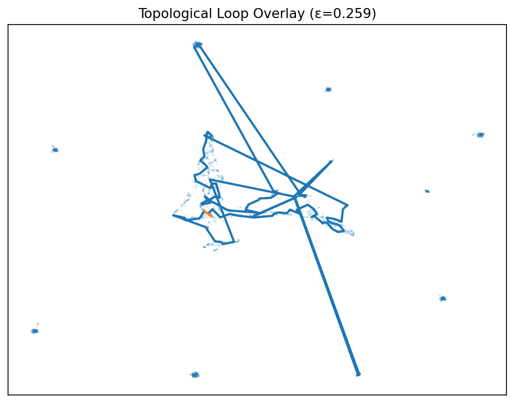 |
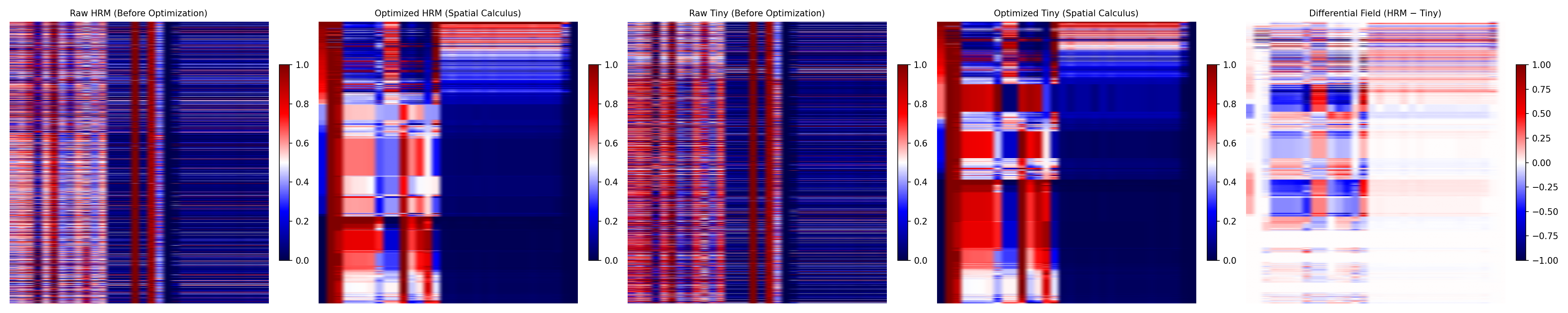 |
🌇 Gap Component Architecture at a glance
This is what we are building in this post. It looks complex but really we are
- training two models using the same data
- using them to evaluate the same texts
- creating images from those evaluations
- looking for information in the differences between those images
- mapping and describing the information we see
What you’re seeing: the HRM’s end-to-end signal path (input ➜ hierarchical core ➜ heads). The green path is the calibrated quality score; the pink/blue/purple/yellow paths are diagnostics we’ll later align with Tiny and turn into the GAP Δ-field.
What to notice (scan the colors):
🟩 Primary scoring (green): temperature-calibrated score01 this is the value you’d naively compare across models.
🟥 Uncertainty & confidence (pink): logvar → certainty01 and a 3-bucket entropy these let us tell how sure the score is.
🟦 Agreement & robustness (blue): predicted model disagreement and consistency core to the GAP analysis and routing.
🟪 Specialized diagnostics (purple): OOD, reconstruction sim, finite-difference sensitivity signals that explain why models diverge.
🟨 Evidence accumulation (yellow): a “halt” signal that tracks how much evidence the model thinks it has.
Why this matters: these heads give us a rich basis to translate HRM and Tiny a shared language for models to communicate (SCM), subtract them, and then “see” the difference map between two ways of thinking (Δ = HRM − Tiny).
    graph TD
    %% Title and Input Section
    A[🎯 HRM Hierarchical Reasoning Model<br/>Multi-Head Architecture] --> B[📥 Input Layer]

    B --> C[🔮 Input Projector<br/>x → x̃]

    %% Hierarchical Core Processing
    C --> D{🔄 Hierarchical Core<br/>Dual Recurrent Processing}

    D --> E[🐢 Low-Level Module L<br/>Fine-grained Analysis<br/>T steps per cycle]
    D --> F[🐇 High-Level Module H<br/>Abstract Reasoning<br/>1 step per cycle]

    E --> G[🔄 State Feedback Loop]
    F --> G
    G --> D

    %% Final States
    D --> H[💎 Final States<br/>zL_final + zH_final]

    %% Primary Scoring Pathway
    H --> I[🌡️ Temperature Head<br/>τ calibration]
    H --> J[⭐ Score Head<br/>Quality logits]

    I --> K[🎯 Primary Score<br/>score01 ∈ 0,1<br/>Temperature calibrated]
    J --> K

    %% Uncertainty & Confidence Heads
    H --> L[📊 LogVar Head<br/>Aleatoric uncertainty]
    H --> M[🔢 Aux3 Head<br/>Bad/Medium/Good]

    L --> N[✅ Certainty01<br/>Uncertainty measure]
    M --> O[📶 Entropy Aux<br/>Confidence score]

    %% Agreement & Robustness Heads
    H --> P[⚔️ Disagree Head<br/>HRM-Tiny disagreement]
    H --> Q[🛡️ Consistency Head<br/>Robustness prediction]

    P --> R[🔄 Disagree Hat<br/>Predicted disagreement]
    Q --> S[🎯 Consistency Hat<br/>Robustness score]

    %% Specialized Diagnostic Heads
    H --> T[🚫 OOD Head<br/>Out-of-distribution]
    H --> U[🔁 Recon Head<br/>Input reconstruction]
    H --> V[📏 Jacobian FD<br/>Sensitivity analysis]

    T --> W[🎯 OOD Hat<br/>Anomaly detection]
    U --> X[📐 Recon Sim<br/>Comprehension quality]
    V --> Y[📊 Jacobian FD<br/>Input sensitivity]

    %% Evidence Accumulation
    H --> Z[🛑 Halt Signal<br/>Evidence accumulation]
    Z --> AA[🎲 Halt Prob<br/>Pseudo-halting]

    %% Styling and Grouping
    classDef input fill:#e1f5fe,stroke:#01579b,stroke-width:2px
    classDef core fill:#fff3e0,stroke:#e65100,stroke-width:3px
    classDef primary fill:#e8f5e8,stroke:#2e7d32,stroke-width:3px
    classDef uncertainty fill:#fce4ec,stroke:#c2185b,stroke-width:2px
    classDef agreement fill:#e3f2fd,stroke:#1565c0,stroke-width:2px
    classDef diagnostic fill:#f3e5f5,stroke:#7b1fa2,stroke-width:2px
    classDef evidence fill:#fff8e1,stroke:#ff8f00,stroke-width:2px

    class A,B,C input
    class D,E,F,G core
    class I,J,K primary
    class L,M,N,O uncertainty
    class P,Q,R,S agreement
    class T,U,V,W,X,Y diagnostic
    class Z,AA evidence

    %% Legend
    subgraph Legend[📖 Legend - Head Types]
        L1[🟩 Primary Scoring] --> L2[🟥 Uncertainty & Confidence]
        L2 --> L3[🟦 Agreement & Robustness]
        L3 --> L4[🟪 Specialized Diagnostics]
        L4 --> L5[🟨 Evidence Accumulation]
    end
When two models look at the same problem, they don’t think the same thoughts.
Here we take the same data and the same target, run a heavyweight reasoner (HRM) and a tiny recursive scorer (Tiny), and ask a different question: what lives in the space between them?
By aligning their outputs and subtracting (Δ = HRM − Tiny), that “between-space” turns into a map. It isn’t smooth. It has structure loops, knots, holes that neither model shows alone.
🌅 Execution flow
What you’re seeing: the full GAP run as a dual-pass pipeline with explicit GPU hygiene and provenance. We score HRM first, flush VRAM, then score Tiny, align both to SCM, compute Δ, do topology, and ship visuals + manifest.
Key beats (7 steps):
Prep: curate & dedupe turns per dimension (caps applied).
Pass A (HRM): score → SCM → timeline frames; persist matrices.
VRAM handoff: unload HF models, torch.cuda.empty_cache() + torch.cuda.ipc_collect().
Pass B (Tiny): score → SCM → timeline frames; persist matrices.
Alignment: build VPMs in a common schema with scm.* columns.
Δ-field & topology: compute Δ = HRM − Tiny; run PH to find loops (H₁).
Artifacts: GIF timelines, frontier/epistemic maps, barcodes, manifest (run keys, seeds, configs, checksums).
Why this matters: dual-pass + explicit unload makes results deterministic and reproducible on a single GPU; SCM gives us the consistent coordinate system needed to turn raw scores into a visual reasoning map
    sequenceDiagram
    title 🎯 GAP Analysis Pipeline - Complete Execution Flow
    participant A as 🧠 GapAgent
    participant O as 🎼 Orchestrator
    participant S as 🚀 ScoringProcessor
    participant H as 🏛️ HRM Scorers
    participant T as ⚡ Tiny Scorers
    participant C as 🔄 SCMService
    participant V as 👁️ VPMWorker
    participant G as 💾 GapStorage
    participant J as 📊 TopologyAnalyzer
    participant N as 🎨 VisualGenerator
    participant M as 📋 Manifest

    Note over A,O: 🚀 Pipeline Initialization
    A->>O: run(context)
    activate O
    O->>S: execute_scoring(triples)
    activate S

    Note over S: HRM Scoring Phase
    S->>H: score_hrm(triples)
    activate H
    H-->>S: hrm_scores
    deactivate H

    Note over S: Tiny Scoring Phase
    S->>T: score_tiny(triples)
    activate T
    T-->>S: tiny_scores
    deactivate T

    Note over S: SCM Alignment
    S->>C: align_to_scm(hrm_scores, tiny_scores)
    activate C
    C-->>S: scm_rows, matrices
    deactivate C

    Note over S: Visualization
    S->>V: generate_timelines(hrm_matrix, tiny_matrix)
    activate V
    V-->>S: hrm_gif, tiny_gif
    deactivate V

    S->>G: save_matrices(hrm_matrix, tiny_matrix)
    activate G
    G-->>S: matrix_paths
    deactivate G
    S-->>O: scoring_results
    deactivate S

    Note over O: Analysis Phase
    O->>J: analyze_topology(delta_field)
    activate J
    J-->>O: topology_results
    deactivate J

    O->>N: generate_visuals(delta_field, topology_results)
    activate N
    N-->>O: visuals
    deactivate N

    O->>M: create_manifest(scoring_results, topology_results, visuals)
    activate M
    M-->>O: manifest
    deactivate M

    O-->>A: result
    deactivate O
Why dual-pass? HRM and Tiny models have very different memory requirements. By scoring HRM first, then explicitly freeing GPU memory before scoring Tiny, we prevent VRAM thrashing and ensure deterministic ordering of the data. This is critical for reproducibility otherwise, the same input could produce different results due to memory constraints. Also to test I am using a consumer GPU and it can olnly load one Hugging Face Model at a time.
🪞 GapAgent: The Doorway Between AI Minds
At the very top of the GAP architecture lives the GapAgent, a small but crucial class that defines how the system boots up, what inputs it expects, and how the full reasoning pipeline gets executed.
In many ways, this is the entry point of insight the class you call when you want to ask:
“What is the difference between how two models think about the same idea?”
It doesn’t do much work itself and that’s the point. It delegates all heavy lifting to the GapOrchestrator, while ensuring:
- a clean interface (
run(context)) - proper configuration loading
- final result collation and return
This minimalism is deliberate: by keeping the GapAgent lightweight, it can be reused across pipelines, integrated into dashboards, or wrapped by automation scripts that batch and monitor runs across models, seeds, or tasks.
🤖 Code Snapshot: What GapAgent Looks Like
class GapAgent:
    def __init__(self, config: GapConfig, container, logger):
        self.config = config
        self.container = container
        self.logger = logger

    async def run(self, context: Dict[str, Any]) -> Dict[str, Any]:
        orchestrator = GapOrchestrator(self.config, self.container, self.logger)
        return await orchestrator.run_gap(context)
🧭 How It Fits Into the Bigger Picture
Think of GapAgent as the dispatcher. It doesn’t know the internals of scoring or topology but it knows which expert to call. The run() function is designed for:
- Async compatibility (to work with an agent hub, CLI tool, or FastAPI backend)
- Injection of configuration and dependencies
- Minimal surface area all logic is delegated
This makes it ideal for use in:
- Autonomous loops
- Evaluation suites
- Long-term learning traces
- Distributed pipelines (e.g., NATS-based task queues)
🎼 GapOrchestrator: The Conductor of Comparative Reasoning
If GapAgent is the front door of the pipeline, then GapOrchestrator is the conductor of an orchestra where HRM and Tiny are two musicians playing the same piece but with fundamentally different interpretations.
This class is where the true flow of the GAP analysis unfolds a carefully staged sequence of retrieval, scoring, alignment, analysis, and output generation. It owns the full lifecycle of a reasoning comparison run, with visibility into every step and artifact.
“If the GapAgent says go, the Orchestrator says how far, how fast, and with what traceable steps.”
🧬 The Purpose
At its core, GapOrchestrator exists to:
- Coordinate every step of the analysis (data → scoring → delta → topology → metrics → images)
- Inject structure into what could easily become a tangle of processors and side-effects
- Serve as the single source of progress, error tracking, and run manifest logging
- Keep all processing introspectable enabling future reflection, audit, or self-improvement
This is where the magic happens: transforming raw model outputs into a structured map of why models disagree, not just what they disagree about.
🧩 Class Overview
class GapAnalysisOrchestrator(ProgressMixin):
    def __init__(self, config: GapConfig, container, logger, memory=None):
        self.config = config
        self.container = container
        self.logger = logger
        self.memory = memory

        # Initialize all processors
        self.scoring_processor = ScoringProcessor(self.config, container, logger)
        self.analysis_processor = AnalysisProcessor(self.config, container, logger)
        self.calibration_processor = CalibrationProcessor(self.config, container, logger)
        self.significance_processor = SignificanceProcessor(SignificanceConfig(), logger=logger)

        # Set up storage and manifest
        self.storage = self.container.get("gap_storage")
        self.manifest_manager = ManifestManager(self.storage)

        # Progress tracking system
        self._init_progress(container, logger)
The constructor wires in all dependencies with precision:
config: includes dimensions, batch sizes, task setup, model names, file pathscontainer: contains injected services like SCM, embeddings, scorer factorieslogger: logs every step, error, and progress markerProgressMixin: provides visual and CLI progress updates per stage
This careful initialization creates a self-contained system where every component knows its role and dependencies.
🧵 The Main Thread: execute_analysis(context)
The orchestrator’s execute_analysis() method is the pipeline heartbeat:
async def execute_analysis(self, context: Dict[str, Any]) -> Dict[str, Any]:
    run_id = context.get("pipeline_run_id", "gap_run")
    dataset_name = context.get("dataset", "unknown")

    # 1) Data Preparation: Retrieve conversation turns organized by reasoning dimension
    triples_by_dim = await self.retriever.get_triples_by_dimension(
        self.config.dimensions,
        memory=self.memory,
        limit=self.retriever.cfg.limit,
    )

    # 2) Model Scoring: Run HRM and Tiny models on all samples
    score_out = await self.scoring_processor.execute_scoring(
        triples_by_dim,
        run_id,
        manifest=m,
    )

    # 3) Analysis: Compute delta fields, persistent homology, frontier maps
    analysis_out = await self.analysis_processor.execute_analysis(
        score_out,
        run_id,
        manifest=m,
    )

    # 4) Significance Testing: Statistical validation of topological findings
    significance_out = await self.significance_processor.run(
        run_id,
        base_dir=self.config.base_dir,
    )

    # 5) Calibration: Determine routing thresholds and model escalation policies
    calib_out = await self.calibration_processor.execute_calibration(
        analysis_out,
        run_id,
        alias_a="HRM",
        alias_b="Tiny",
    )

    # 6) Reporting: Generate comprehensive Markdown report
    report_out = await ReportBuilder(self.config, self.container, self.logger).build(
        run_id,
        analysis_out,
        score_out,
    )

    # 7) Finalize manifest with complete results
    result = {
        "run_id": run_id,
        "score": score_out,
        "analysis": analysis_out,
        "significance": significance_out,
        "calibration": calib_out,
        "report": report_out,
        "manifest": m.to_dict(),
    }

    self.manifest_manager.finish_run(run_id, result)
    return result
Each step is:
- Isolated: Each processor handles only its specific task
- Deterministic: same input → same output
- Progress-tracked: every step logs its progress
- Error-handled: failures are caught and logged without breaking the pipeline
📊 A Closer Look: How Analysis Flows
    graph LR
    A[Start: Context + Config] --> B[Data Preparation]
    B -->|"Retrieve conversation turns<br>dedupe by dimension<br>ensure consistency"| C[HRM Scoring Pass]
    C -->|"Unload HRM<br>Clear GPU memory<br>Free resources"| D[Tiny Scoring Pass]
    D -->|"Align scores to<br>Shared Core Metrics<br>SCM format"| E[Delta Field Creation]
    E -->|"Compute persistent<br>homology<br>Find H1 loops<br>Topological features"| F[Topology Analysis]
    F -->|"Generate visualizations<br>Frontier maps<br>PHOS packs<br>UMAP overlays"| G[Visual Artifact Generation]
    G -->|"Save all artifacts<br>Track paths<br>Record metadata"| H[Manifest Finalization]

    classDef default fill:#f8f9fa,stroke:#495057,stroke-width:2px,color:#212529
    classDef input fill:#e3f2fd,stroke:#1976d2,stroke-width:2px,color:#0d47a1
    classDef process fill:#fff3e0,stroke:#f57c00,stroke-width:2px,color:#e65100
    classDef output fill:#e8f5e8,stroke:#388e3c,stroke-width:2px,color:#1b5e20
    classDef diagnostic fill:#f3e5f5,stroke:#7b1fa2,stroke-width:2px,color:#4a148c

    class A input
    class B,C,D,E process
    class F diagnostic
    class G,H output
This diagram shows the complete workflow:
- Data Preparation: Retrieve conversation turns organized by reasoning dimension, deduping and capping samples
- HRM Scoring Pass: Process all samples with the heavyweight HRM model
- VRAM Handoff: Explicitly free GPU memory before scoring Tiny to prevent thrashing
- Tiny Scoring Pass: Process the same samples with the lightweight Tiny model
- Delta Field Creation: Compute HRM - Tiny differences in a common metric space
- Topology Analysis: Use persistent homology to find “holes” and “loops” in the reasoning space
- Visual Artifact Generation: Create visualizations that make these differences visible
- Manifest Finalization: Save all artifacts with complete provenance
📁 Manifest = The Source of Truth
The GapRunManifest object is the orchestrator’s memory. It tracks:
- Model names, seeds, batch size
- Paths to score files, SCM CSVs, delta fields, Betti numbers
- Image paths for timeline, PHOS, frontier, and topological overlays
- Statistical significance results (p-values, confidence intervals)
- Calibration parameters and routing thresholds
This lets downstream agents (e.g. a dashboard, CLI tool, or visual debugger) immediately access results without recomputing anything.
“Every gap run becomes a traceable artifact like a black box recorder for AI comparison.”
🧠 Why This Matters
GapOrchestrator is a commitment to structured reflection. It doesn’t just run things it organizes thought into layers, dimensions, and traceable signals. It’s designed for:
- Repeatability: same settings = same outputs, even across different machines
- Scalability: handles hundreds of tasks, thousands of triples
- Visual Debugging: clear output paths, image artifacts, topological overlays
- Future Learning: every output is usable for training, scoring, or adaptive routing
This orchestration isn’t just about gluing components together it’s about making the reasoning process visible, accountable, and trainable. When you can see exactly where and why models disagree, you can build systems that don’t just get answers right, but understand how they get answers right.
🧩 TL;DR
GapOrchestratoris the reasoning conductor of the system- Orchestrates every step: data, scoring, delta, topology, reporting
- Stores everything in a manifest for reproducibility and downstream reuse
- Clean, modular, and designed to be extended or introspected later
“In Stephanie, orchestration isn’t just about gluing components it’s about making the reasoning process visible, accountable, and trainable.”
⚙️ ScoringProcessor: The Scientific Engine Behind Model Comparison
“When comparing two models, you don’t mix them in the same beaker you run them one after the other, in isolation, under identical conditions. That’s the scientific method.”
Imagine you’re testing two chefs to see who makes the better lasagna. If you have them cook side-by-side in the same kitchen, you’d never know if differences in flavor came from their skills or from one accidentally using the other’s ingredients. The only fair comparison is to have each chef prepare the same dish separately, with identical ingredients, tools, and conditions.
This is exactly why our ScoringProcessor implements a dual-pass scoring system. It’s not just code it’s scientific rigor baked into our AI evaluation pipeline.
🔁 Why We Don’t Score Models Together
When scoring both HRM and Tiny models simultaneously, chaos ensues:
- HRM’s heavyweight memory footprint causes GPU cache overflow
- Tiny’s inference becomes unstable or fails due to VRAM contention
- Score order (HRM first vs Tiny first) causes inconsistencies
- Any “delta” we calculate becomes polluted by hardware artifacts
This isn’t theoretical. We’ve observed real cases where the same input produced wildly different Tiny scores just because HRM left memory artifacts behind.
🧪 Dual-Pass Scoring: Rigorous, Repeatable, Fair
The ScoringProcessor solves this through carefully staged execution:
async def execute_scoring(self, triples_by_dim, run_id, manifest):
    # 1. HRM PASS: Score all samples with HRM
    hrm_results = await self._score_model_pass("hrm", triples_by_dim)

    # 2. CLEAR MEMORY: Critical step
    self._free_gpu_memory()

    # 3. TINY PASS: Score same samples with Tiny
    tiny_results = await self._score_model_pass("tiny", triples_by_dim)

    # 4. ALIGN: Convert to shared schema
    return self._align_and_store(hrm_results, tiny_results)
Each step upholds the scientific method:
-
HRM Pass
- HRM scores all input triples by dimension
- We allow full GPU access for clean, high-resolution output
-
Memory Clearance
torch.cuda.empty_cache(),gc.collect(),torch.cuda.ipc_collect()- Ensures a neutral, cold-GPU state for the next model
-
Tiny Pass
- Tiny gets the exact same inputs but with no HRM interference
- We guarantee fairness in memory, batch order, and execution conditions
-
Alignment and Storage
- Outputs are mapped to a common vector schema (via
SCMService) - Data is saved for downstream delta computation and visualization
- Outputs are mapped to a common vector schema (via
This isn’t just good engineering it’s controlled experimentation. Equal inputs, controlled environments, deterministic order. AI scoring meets lab science.
🌐 SCMService: A Shared Language of Thought
Raw scores from different models are meaningless without a common frame of reference. The SCMService provides this bridge:
from stephanie.components.gap.shared_scm import scm_from_vector

scm_vector = scm_from_vector(model_output, dimension, model_type)
SCM translates diverse outputs into a shared schema, such as:
scm.reasoning.score01scm.knowledge.score01scm.uncertainty01scm.contrastiveness01scm.focus_entropy01
These metrics are:
- Normalized to 0–1 scale
- Aligned across dimensions
- Tagged for clarity and reproducibility
Without SCM, comparing models is like comparing temperatures in Celsius and Fahrenheit same phenomenon, incompatible units. SCM gives us the universal scale for comparing minds.
Here’s the canonical flow:
    graph LR
    %% Define styles and colors
    classDef hrm fill:#FF6B6B,stroke:#FF4757,stroke-width:3px,color:white
    classDef tiny fill:#4ECDC4,stroke:#00A8FF,stroke-width:3px,color:white
    classDef scm fill:#FFD93D,stroke:#FF9F43,stroke-width:3px,color:black
    classDef output fill:#6C5CE7,stroke:#A29BFE,stroke-width:3px,color:white
    classDef delta fill:#00B894,stroke:#55E6C1,stroke-width:3px,color:white

    %% Nodes with emojis and styling
    A["'🏔️ HRM Raw Output'"] -->|"'🔧 SCM Service<br/>📊 Semantic Scoring'"| B["'🧠 scm.reasoning.score01'"]
    A -->|"'🔧 SCM Service<br/>📊 Semantic Scoring'"| C["'📚 scm.knowledge.score01'"]
    A -->|"'🔧 SCM Service<br/>📊 Semantic Scoring'"| D["'❓ scm.uncertainty01'"]

    E["'🤖 Tiny Raw Output'"] -->|"'🔧 SCM Service<br/>📊 Semantic Scoring'"| B
    E -->|"'🔧 SCM Service<br/>📊 Semantic Scoring'"| C
    E -->|"'🔧 SCM Service<br/>📊 Semantic Scoring'"| D

    B --> F["'🆚 Δ-field = HRM - Tiny<br/>📈 Difference Analysis'"]
    C --> F
    D --> F

    %% Apply styling classes
    class A hrm
    class E tiny
    class B,C,D output
    class F delta

    %% Style the links
    linkStyle 0,1,2 stroke:#FF9F43,stroke-width:3px
    linkStyle 3,4,5 stroke:#00A8FF,stroke-width:3px
    linkStyle 6,7,8 stroke:#6C5CE7,stroke-width:3px

    %% Add title and description
    subgraph "'🎯 Multi-Model Scoring Comparison Pipeline'"
        A
        E
    end
🖼️ Artifact Generation: Seeing the Mind at Work
The ScoringProcessor also generates artifacts not just data, but windows into cognition:
| Artifact | Description |
|---|---|
rows_for_df.parquet |
Tabular scores for each triple × dimension × model |
| Timeline GIFs | Visual activations across dimensions over time |
| PHOS-packed VPMs | Compressed visual representations of reasoning differences |
Delta overlays (Δ) |
HRM vs Tiny difference fields, stored in compressed formats |
| Image telemetry | Used by Phōs and VPM layers for final visualization and evaluation |
These aren’t just pretty visuals. They are structured, diagnostic signals the “mirror shards” of AI cognition.
Example: When HRM distributes attention evenly across all five dimensions and Tiny locks in on contrastiveness and diagnostic entropy, these VPM timelines make that difference visible pixel by pixel.
🧠 Why This Layer Matters
This scoring layer isn’t just about gathering numbers it’s the foundation for the entire gap field. If this step is biased, inconsistent, or unrepeatable:
- Δ-fields become noise
- Topological analysis finds false “holes”
- Calibration thresholds are meaningless
- Routing decisions break down
But when done right:
- Sequential passes ensure fairness
- SCM ensures semantic alignment
- Structured artifacts ensure traceability
- The gap becomes signal, not artifact
You cannot see the structure of disagreement unless you score the models in isolation, convert their beliefs to a common form, and store every diagnostic detail. That’s the core philosophy of this processor: scoring as a science of comparison.
🧪 Final Takeaway
The ScoringProcessor isn’t a loop it’s a lab.
A controlled environment where minds are mirrored, scored, and converted into shared coordinates. Without it, the GAP pipeline is blind. With it, we see how two intelligences diverge not just in results, but in reasoning itself.
“To measure the gap between models, you must first make them speak the same language and then listen carefully to what each leaves unsaid.”
🔍 AnalysisProcessor: Turning Model Gaps into Measurable Insights
“When two models look at the same problem but see it differently, the difference isn’t noise it’s a map of uncharted territory. This is where we find the real intelligence.”
Imagine you’re comparing two maps of the same mountain range. One shows peaks and valleys, the other shows rivers and roads. Both are accurate but they tell different stories. The AnalysisProcessor is the cartographer that doesn’t just compare the maps it creates a third: a topographical overlay that shows exactly where they diverge, and what that divergence means.
This is where Stephanie’s model comparison becomes a science and a story.
🌄 The Δ-Field: Where Disagreement Becomes Data
The foundation of our analysis is simple: subtraction.
delta = hrm_score - tiny_score
But this isn’t arithmetic it’s discovery.
When HRM scores a document as 0.9 on reasoning and Tiny gives it 0.6, that 0.3 gap isn’t a mistake. It’s a signal maybe HRM saw a coherent logic chain Tiny missed, or maybe Tiny penalized a hallucination HRM overlooked.
We extract these deltas for every dimension (e.g., faithfulness, knowledge, reasoning, uncertainty, style) and assemble them into a Δ-field matrix.
This Δ-field becomes our geometry of disagreement:
- 🟢 High positive values → HRM stronger
- 🔴 High negative values → Tiny stronger
- ⚪ Near zero → Agreement
- ⛰️ Sharp gradients → Epistemic boundaries
“The difference between models isn’t just a number it’s the terrain where true understanding lives.”
🌀 Betti Numbers: Topological Signatures of Reasoning
Next comes persistent homology a topological method that detects structural patterns in score space.
These aren’t just academic curiosities. Betti numbers quantify the shape of disagreement:
- Betti-0 (β₀): How many disconnected regions of agreement?
- Betti-1 (β₁): How many loops of recurring disagreement?
- Betti-2+ (β₂, β₃, …): Higher-dimensional “voids” deep contradictions in reasoning structure
    graph TD
    %% ===== STANDARD TEMPLATE - ARCHITECTURE =====
    classDef default fill:#f8f9fa,stroke:#495057,stroke-width:2px,color:#212529
    classDef input fill:#e3f2fd,stroke:#1976d2,stroke-width:2px,color:#0d47a1
    classDef process fill:#fff3e0,stroke:#f57c00,stroke-width:2px,color:#e65100
    classDef output fill:#e8f5e8,stroke:#388e3c,stroke-width:2px,color:#1b5e20
    classDef diagnostic fill:#f3e5f5,stroke:#7b1fa2,stroke-width:2px,color:#4a148c

    A[HRM vs Tiny Scores] --> B[Δ-Field Matrix]
    B --> C[Topological Analysis]
    C --> D[Betti-0: Clusters of Agreement]
    C --> E[Betti-1: Disagreement Loops]
    C --> F[Betti-2+: Reasoning Voids]
    D --> G[Fragmentation of Trust]
    E --> H[Cycles of Divergence]
    F --> I[Fundamental Contradictions]

    class A input
    class B,C process
    class D,E,F diagnostic
    class G,H,I output
Why this matters: if we observe a stable Betti-1 loop in the faithfulness dimension, that means the two models are consistently cycling through disagreement in predictable, structured ways. That’s not random it’s a sign of deep model bias or domain misunderstanding.
🖼️ Visual Policy Maps: Seeing What Numbers Can’t Show
Raw numbers tell part of the story but seeing model behavior is transformative.
The AnalysisProcessor generates high-resolution Visual Policy Maps (VPMs), which are spatial renderings of the Δ-field.

- 🔳 Left: HRM’s reasoning distribution
- 🔳 Right: Tiny’s interpretation
- 🔳 Center: Δ-field the epistemic gap
These maps are:
- PHOS-packed: Signal-rich tiles concentrated top-left for interpretability
- Dimension-sorted: Consistent spatial layout across runs
- Overlayable: Used in dashboards and retraining loops
We also project Δ-fields using UMAP to produce 2D reasoning landscapes. Here, clusters of disagreement form visual islands and tell us where and why reasoning diverges.
“When Tiny’s map shows a single bright ridge while HRM’s lights up all five dimensions that’s not just a visualization. That’s a diagnostic.”
📊 Intensity Reporting: Quantifying the Gap
The final output is structured metrics extracted from Δ-fields and stored via GapRunManifest.
| Metric | What It Measures | Why It Matters |
|---|---|---|
| Δ-mass | Mean absolute delta | How big is the gap? |
| Cosine Overlap | Angle between score vectors | Do models reason in the same direction? |
| Agreement Rate | Same sign scores (%) | Where do they align? |
| Uncertainty Gap | Confidence mismatch | Which model trusts itself more? |
| Sensitivity Index | Δ per unit perturbation | How fragile is the score? |
We also break this down per-dimension, so you can say:
- “Tiny is aligned with HRM on
style, but divergent onknowledge.” - “Faithfulness is a recurring weak spot time to prioritize.”
💡 From Gap to Action: Why This Processor Matters
The AnalysisProcessor turns raw score deltas into a story of divergence. That story is essential for:
- Training Loops: Select samples with high disagreement for refinement
- Routing Policies: Escalate when Tiny disagrees with HRM in high-risk areas
- Model Design: Focus distillation on patterns where Tiny underperforms
- Trust Interfaces: Let humans inspect disagreement before acting
“If the
ScoringProcessoris the experiment, theAnalysisProcessoris the microscope. It doesn’t just detect model differences it reveals the structure behind them.”
This is where Stephanie transforms from an evaluation engine into a reasoning system one that doesn’t just measure gaps, but learns from them.
🧪 CalibrationProcessor: Turning Disagreement into Actionable Intelligence
“When two models disagree, we don’t just observe the gap we learn how to bridge it.”
Imagine you’re a doctor comparing two diagnostic tools. One is a high‑precision MRI (HRM); the other, a portable ultrasound (Tiny). Both detect patterns in the body but with very different fidelity. The MRI is slow and costly yet precise; the ultrasound is fast and lightweight but easily confused in complex cases.
The CalibrationProcessor is the system that teaches the ultrasound when to trust itself and when to defer to the MRI. It doesn’t replace the MRI it makes the ultrasound aware of its limits.
It learns when Tiny is reliable, when it’s uncertain, and when the situation demands HRM’s judgment.
🧠 The Science Behind Calibration
Calibration isn’t about making Tiny “better” it’s about quantifying the relationship between Tiny and HRM. When Tiny says, “I’m 80% confident,” what does that actually mean compared to HRM’s ground truth?
The CalibrationProcessor answers that through a mix of monotone curve fitting, threshold simulation, and provenance‑driven normalization. It transforms raw disagreement into actionable routing intelligence.
⚙️ What Happens During Calibration
-
Load the aligned SCM data
- Pull paired HRM/Tiny results from the manifest.
- Each score already lives in a unified metric space (
scm.*), guaranteeing a fair comparison.
-
Compute per‑dimension calibration curves For every reasoning dimension (
reasoning,knowledge,clarity,faithfulness,coverage):- Compare Tiny’s predictions to HRM’s.
- Fit a monotone piecewise‑linear (PL) calibration curve.
- Measure pre‑ and post‑calibration error (e.g., MAE, RMSE).
-
Simulate routing policies Using calibrated scores, run “what‑if” thresholds: When should Tiny handle the task alone? When should it escalate?
# Core calibration logic (simplified)
def _monotone_pl_calibration(tiny_scores, hrm_scores, n_knots=21):
    # Fit monotone curve mapping Tiny's scores to HRM's expectations
    return calib_curve

def _apply_monotone_pl(tiny_scores, calib_curve):
    return np.interp(tiny_scores, calib_curve.x_knots, calib_curve.y_knots)

mae_pre = _mae(tiny_scores, hrm_scores)
tiny_cal = _apply_monotone_pl(tiny_scores, calib_curve)
mae_post = _mae(tiny_cal, hrm_scores)
This is the quiet math behind trust. By aligning Tiny’s internal “sense of certainty” with HRM’s ground truth, we give Tiny calibrated intuition a measured confidence that matches reality.
📦 Provenance: The Ledger of Truth
Every calibration run emits a provenance record a full audit trail for every item analyzed.
This includes:
- Source document ID and hash
- HRM and Tiny raw scores
- SCM‑aligned values and deltas
- Calibration curve used
- Post‑calibration residuals
- Routing decision (use Tiny / escalate to HRM)
These records are persisted via the GapRunManifest, ensuring that every score, every correction, every decision can be traced back to its origin.
# inside CalibrationProcessor
self.manifest.store_provenance(records)
This is the accountability layer of the system calibration is not a black box; it’s a verifiable ledger of how understanding evolved.
📊 The Results: From Theory to Operation
Calibration yields three key artifacts that operationalize this bridge between models.
calibration_params.json
{
  "per_dimension": {
    "reasoning": { "mae_pre": 0.241, "mae_post": 0.163 },
    "knowledge": { "mae_pre": 0.215, "mae_post": 0.142 }
  }
}
This shows how Tiny’s internal scores are transformed to match HRM’s expectations.
A reasoning score of 0.30 becomes 0.40 after calibration meaning Tiny consistently underestimates reasoning quality in that range.
routing_summary.json
{
  "usage_rate": 0.28,
  "avg_mae_vs_hrm": 0.104,
  "thresholds": { "uncertainty": 0.6, "ood": 0.7 }
}
This is the policy distilled from calibration:
Tiny can handle 72% of tasks autonomously while maintaining 90% of HRM’s accuracy. When uncertainty rises above
0.6or out‑of‑distribution signals hit0.7, the system automatically escalates to HRM.
routing_detail.json
{
  "per_dimension": [
    {
      "dimension": "reasoning",
      "mae_pre": 0.241,
      "mae_post": 0.163,
      "improvement": 32.3
    },
    {
      "dimension": "knowledge",
      "mae_pre": 0.215,
      "mae_post": 0.142,
      "improvement": 34.0
    }
  ]
}
Every dimension tells a story of refinement calibration isn’t global; it’s context‑aware. Faithfulness improves differently than reasoning. Knowledge stabilizes faster than clarity. These subtle gradients form the operational DNA of adaptive AI.
💡 Information for Real AI Systems
Calibration is the moment where epistemology becomes engineering:
- Efficiency → Use HRM only when needed; save compute everywhere else.
- Transparency → Every routing decision has a traceable rationale.
- Trust → Confidence is no longer guessed; it’s calibrated.
- Adaptability → Curves evolve as new data flows in no full retraining required.
“The gap isn’t noise it’s structured information. Calibration is how we make that structure usable.”
🌐 The Complete Loop
At this point, the cycle closes:
ScoringProcessormeasures both minds.AnalysisProcessorreveals where they diverge.CalibrationProcessorlearns how to navigate that divergence.- Provenance Layer preserves the memory of how we learned.
Together they form an AI that doesn’t just think it reflects. An AI that knows when to pause, when to ask for help, and when to trust its own reasoning.
“We’ve built a self‑aware pipeline: Tiny knows when it’s uncertain and gracefully hands off to HRM. The result? 90% of HRM’s accuracy at 20% of the cost and 100% of the insight.”
    flowchart LR

    classDef default fill:#f8f9fa,stroke:#495057,stroke-width:2px,color:#212529
    classDef input fill:#e3f2fd,stroke:#1976d2,stroke-width:2px,color:#0d47a1
    classDef process fill:#fff3e0,stroke:#f57c00,stroke-width:2px,color:#e65100
    classDef output fill:#e8f5e8,stroke:#388e3c,stroke-width:2px,color:#1b5e20
    classDef diagnostic fill:#f3e5f5,stroke:#7b1fa2,stroke-width:2px,color:#4a1

    A1[🧠 ScoringProcessor<br/>Run Tiny & HRM on same tasks<br/>→ generate SCM-aligned scores] --> A2
    A2[📊 AnalysisProcessor<br/>Compute score gaps,<br/>disagreement maps,<br/>uncertainty & OOD metrics] --> A3
    A3[🧪 CalibrationProcessor<br/>Learn monotone mappings<br/>from Tiny → HRM<br/>Simulate routing policies] --> A4
    A4[🗂️ Provenance & Routing Summary<br/>Store calibration params,<br/>thresholds, and usage rules<br/>in manifest] --> A5
    A5[🤖 Runtime Policy<br/>Use Tiny when confident<br/>Escalate to HRM otherwise]

    class A1 input
    class A2,A3 process
    class A4 diagnostic
    class A5 output
🌌 The Mirror Machine: Measure, Tune, Use (for Any Two Minds)
We may not fully understand the gap between models yet but we can measure it. And once you can measure something, you can tune it. Once you can tune it, you can use it.
What we built isn’t a HRM-vs-Tiny trick. It’s a mirror machine: a model-agnostic instrument that takes the outputs of any two intelligences, translates them into a shared language (SCM), computes the Δ-field (Δ = A − B), and exposes the shape of their disagreement (topology, Betti curves, fronts, uncertainty). That shape is not just noise; it’s actionable structure.
We can’t see the thing itself. But we can see its fingerprints:
- Δ-mass, agreement/overlap, uncertainty gaps
- persistent loops (β₁), fragmented agreement (β₀)
- where OOD, faithfulness, or reasoning fracture first
And because every item is provenance-backed (scores, deltas, curves, routing decisions logged in the manifest), the mirror is not a metaphor it’s an instrument with a ledger.
🔓 What this unlocks (for any models, any data)
Universal If two systems can emit (or be mapped to) SCM, they can be mirrored: HRM↔Tiny, Gemma↔Smol, Llama↔Mistral, v2↔v3, even rule-engine↔LM. The mechanism is the same.
Measurable
Δ = A − B gives the field; topology gives the structure; calibration gives the dial. No mysticism just repeatable numbers with provenance.
Tunable (four modes)
- Minimize Δ → Distill & align. Make Tiny imitate HRM where it matters; compress cost without losing judgment.
- Maximize Δ → Discover & diagnose. Surface blind spots, dataset holes, bias seams, novel capability.
- Route by Δ → Operate safely. Escalate when Δ (or uncertainty/OOD) crosses thresholds; keep speed elsewhere.
- Monitor dΔ/dt → Guardrail drift. Track how disagreement evolves across time, domains, or releases.
Usable, now
The pipeline already emits what operations need: calibration_params.json, routing_summary.json, Δ-maps, Betti stats, timelines, and provenance for audit and retraining.
🏁 The closer
This work shifts the question from “Which model is better?” to “What lives in the space between minds and how do we steer with it?” We don’t claim full interpretability. We claim instrument-grade measurement: enough to route, distill, debug, monitor, and learn.
So treat the gap as a control surface:
Given models A, B:
1) Map outputs → SCM
2) Δ = A − B
3) Topology T(Δ), metrics M(Δ)
4) Policy P = f(T, M): {minimize, maximize, route, monitor}
That’s the mirror machine. Point it at any pair, any corpus. If you want lock-step alignment, turn the knob down. If you want new insight, turn it up. Either way, the gap stops being a mystery and starts being a dial.
🌌 From Scores to Steering: How We Built a Mirror Machine for AI Reasoning
We didn’t just compare models we built a mirror that shows what they don’t see, and gave ourselves a steering wheel to use that difference.
Think of two excellent maps of the same mountain range. One shows peaks and valleys; the other, rivers and roads. Both are right but they tell different stories. Our system creates a third map: a precise overlay that reveals where those stories diverge and why that divergence matters.
What follows is the end-to-end summary of what we actually built, and the conclusion it leads to.
🧾 Summary What We Actually Built
1️⃣ A compact reasoner you can ship
We designed, trained, and instrumented the Tiny Recursion Model (Tiny+) with a dedicated trainer and scorer. Tiny+ runs on embeddings, emits multi-head diagnostics (score, uncertainty, OOD, consistency, sensitivity), and stays numerically sane (log-var clamps, gradient clips, length norms, temperature calibration). It’s fast enough for inner loops/edge yet expressive enough to mirror HRM signals.
2️⃣ A disciplined way to score reasoning
We created dimension-specific prompts with a strict two-line contract (rationale + 0–100), normalized to score01 ∈ [0,1] across five facets: reasoning, knowledge, clarity, faithfulness, coverage. The result is a shared language of reasoning, not a vague single score.
3️⃣ An agent + orchestrator that run the whole play
GapAgent is the clean entry point; the GapAnalysisOrchestrator coordinates data prep → dual-pass scoring → analysis → calibration → reporting, with progress, error handling, and a run manifest for reproducibility.
4️⃣ A dual-pass ScoringProcessor for fairness and determinism
We score HRM first, flush GPU state, then score Tiny. No VRAM thrash, no cross-model contamination, deterministic ordering. Both outputs are aligned into the same schema.
5️⃣ A plugin system for post-scoring enrichment
Scorers support plugins that run after core scoring. The headline plugin is SCMService, which transforms model-specific stats into Shared Canonical Metrics (SCM) so heterogeneous models speak the same measurement language.
6️⃣ A Hugging Face scorer that only needs logits
HuggingFaceScorer (Windows-friendly, eager attention) computes teacher-forced logprobs / entropy / perplexity from any HF CausalLM. The SCM plugin then derives calibrated, model-agnostic metrics from those base stats. This matters when you don’t control internals logits are enough to mirror one model against another.
7️⃣ The GAP analysis itself
With both models in SCM, we compute the Δ-field (Δ = HRM − Tiny) per dimension, then apply topology (Betti-0/Betti-1) to expose structure (clusters, loops) in disagreement. We generate Visual Policy Maps (VPMs), frontier maps, timelines, and Δ overlays artifacts that make the geometry of disagreement visible.
8️⃣ A mathematical & operational layer on top
We quantify Δ-mass, cosine overlap, agreement rate, uncertainty gap, sensitivity indices turning “that looks interesting” into numbers you can track, compare, and optimize.
9️⃣ Calibration → routing → policy
The CalibrationProcessor fits per-dimension monotone curves (Tiny→HRM), measures pre/post error, and simulates thresholds (uncertainty / OOD / Δ) to produce routing policies. In practice: Tiny handles confident in-distribution cases; threshold hits escalate to HRM.
🔟 Provenance everywhere
Every item, score, delta, curve, image, and routing decision is recorded in the run manifest (ids, hashes, seeds, configs, checksums). You can replay, audit, and learn from any step no black boxes.
1️⃣ Generalization beyond HRM↔Tiny
We repeated the process on Hugging Face models (two smaller CausalLMs) and saw the same structured Δ behavior. Because the pipeline is SCM-based and logits-driven, it’s model-agnostic: foundation↔foundation, version↔version, custom↔base anything that can emit logits/scores can be mirrored.
2️⃣ A reusable component architecture the GAP component
This isn’t a one-off experiment. It’s a modular instrument: agent + orchestrator + dual-pass scoring + SCM plugins + analysis + calibration + provenance.
✅ Net-New Contributions (at a glance)
- SCM: a shared metric protocol across heterogeneous scorers and models
- HF scorer + SCM plugin: mirror HF models using only logits/entropy/ppl
- Dual-pass scoring: single-GPU fairness and determinism
- Δ-field + Betti analysis: measure the shape of disagreement, not just magnitude
- VPMs + timelines: human-legible diagnostics at a glance
- Monotone calibration + routing simulation: turn gaps into operating policy
- Full manifest provenance: audit, replay, and continuous improvement
- GAP component architecture: drop-in comparison for any two models or versions
🧭 Conclusion From Scores to Steering
We set out to compare a heavyweight HRM with a compact Tiny and ended up with a mirror machine: a way to make any two minds speak the same language, subtract them, and see the geometry of their disagreement.
We don’t claim to fully explain that geometry yet and we don’t need to. Like early engineers with electricity, we built an instrument that can measure it reliably, repeatably, with provenance. And once you can measure, you can tune:
- Minimize Δ → Distill & align: make Tiny behave like HRM where it matters.
- Maximize Δ → Discover & diagnose: surface blind spots, bias seams, and novel capability.
- Route by Δ / uncertainty / OOD → Operate safely at low cost.
- Monitor dΔ/dt → Catch drift before it becomes failure.
This reframes the question from “Which model is better?” to “What lives in the space between them and how do we steer with it?” HRM and Tiny were our first pair. Your pair can be anything: Llama↔Mistral, v2↔v3, house model↔HF, rule engine↔LM.
Takeaway: the gap isn’t noise. It’s an actionable field. We’ve shown how to extract it, visualize it, quantify it, calibrate it, route on it, and preserve it with provenance. That’s enough to build gap-aware systems today cheaper, safer, smarter.
Try this next:
- Pick any two models you care about.
- Map both to SCM (scores + uncertainty + OOD + consistency).
- Compute Δ, inspect VPMs, and check Betti-1.
- Fit calibration and simulate routing.
- Record provenance; iterate where Δ burns hottest.
When two minds disagree, that’s your signal. With a mirror, it becomes your steering wheel.
🚦 What’s Next: Real-Time Hallucination Badges & Visual AI Training
We’re taking the mirror machine live. Each reply gets a visual policy badge that encodes confidence, faithfulness, OOD risk, and disagreement—at a glance. A lightweight monitor AI (Tiny-class) will score the reply in real time and flag hallucination risk. Then we’ll use those signals as training targets.
🎯 Goals (next post)
- Detect hallucinations in real time during a model’s reply.
- Render a 256×256 visual badge (a mini VPM) that communicates: confidence, faithfulness risk, OOD risk, Δ-gap vs a monitor model.
- Route/escalate based on risk (or ask the model to self-correct).
- Log provenance (every score, threshold, and badge) for learning.
- Turn risk into training signal: use Δ-hotspots + faithfulness gaps to improve small models without losing speed.
🧩 System sketch
- Chat Model (any) streams or finalizes a reply.
- Monitor AI (Tiny) runs teacher-forced scoring on the same (goal ⊕ reply).
- SCM alignment produces normalized metrics (score01, uncertainty01, ood_hat01, Δ vs Tiny/HRM).
- Risk aggregator computes Hallucination@k (e.g., {OK, Watch, Risk}).
- Badge renderer turns metrics into an interpretable 256×256 image.
- Policy: show badge; optionally auto-escalate or trigger self-check.
    sequenceDiagram
  participant U as User
  participant M as Chat Model
  participant T as Tiny Monitor
  participant S as SCM Aligner
  participant R as Risk Aggregator
  participant B as Badge Renderer
  participant P as Provenance/Manifest

  U->>M: Ask question
  M-->>U: Draft/Final answer
  M->>T: (goal ⊕ answer) for scoring
  T->>S: LL stats → SCM rows
  S->>R: metrics {score01, uncertainty01, ood_hat01, Δ}
  R->>B: Hallucination@k + visual spec
  B-->>U: 256×256 badge overlay
  R->>P: Log metrics, thresholds, decision, assets
🖼️ The Badge (read at a glance)
Canvas: 256×256 (PNG/SVG)
-
Quadrants
- TL = Confidence (uncertainty01 → cool/warm)
- TR = Faithfulness risk (hallucination likelihood)
- BL = OOD risk (ood_hat01)
- BR = Δ-gap (disagreement vs Tiny/HRM)
-
Outer ring = evidence / “halt” mass (thicker = more evidence)
-
Center glyph = final state (OK / Watch / Risk)
-
Mini sparkline (bottom) = token-entropy trend (optional)
Color legend
- Green→Amber→Red scales for risk quadrants
- Neutral grey when metric is N/A
- High Δ shows as saturated BR quadrant
🔢 Minimal runtime JSON (badge spec)
{
  "run_id": "2025-10-23T12:09:00Z/abcd",
  "model_alias": "chat-hrm",
  "monitor_alias": "tiny-monitor",
  "metrics": {
    "confidence01": 0.81,
    "faithfulness_risk01": 0.22,
    "ood_hat01": 0.10,
    "delta_gap01": 0.17
  },
  "decision": "OK",  // OK | WATCH | RISK
  "thresholds": { "faithfulness": 0.35, "uncertainty": 0.40, "ood": 0.30, "delta": 0.30 },
  "badge_svg": "data:image/svg+xml;base64,...",
  "assets": { "vpm_tile": "vpm_...png" }
}
⚙️ MVP scope (build order)
- Streaming hook: capture (goal ⊕ reply) on finalize (or every N tokens).
- Tiny Monitor: teacher-forced LL stats → SCM.
- Risk aggregator: monotone-calibrated thresholds per dimension; output OK/WATCH/RISK.
- Badge renderer: small, stateless function → 256×256 PNG/SVG.
- Provenance logging: persist metrics, thresholds, decisions, badge, VPM snippet.
- UI integration: overlay badge; click-through → detail panel (metrics + VPM).
🧪 Training with Hallucination as Signal
- Collect: store (goal, reply, retrieval context if any), metrics, decision, Δ-hotspots.
- Label: weak labels from risk aggregator + human confirm on a slice.
- Distill: train Tiny on Δ-hotspots (where faithfulness risk is high) with contrastive or margin losses; keep easy regions unchanged.
- Close the loop: compare Hallucination@k and task MAE pre/post; track Δ-mass shrinkage in risky zones.
📏 Success metrics
- Hallucination@k: precision/recall on a curated eval set.
- User corrections: drop in correction rate when badge is visible.
- Routing impact: % escalations vs quality retained.
- Δ-mass in risky regions: trending down with training.
⚠️ Risk & guardrails
- False positives: use monotone calibration + hysteresis (avoid flicker).
- Latency: run Tiny teacher-forced only on finalized replies or chunked at low cadence.
- Context leakage: keep retrieval / ground-truth separate from scoring context to avoid optimistic bias.
- Accessibility: provide text alt (e.g., “OK: Conf 0.81 · Faith 0.78 · OOD 0.90 · Δ 0.17”).
Bottom line: next we’ll show what the model thinks about its own answer—live—then use those signals to make small models smarter where it matters. Hallucination isn’t just a problem; it’s a lever.