12: The Closest Thing We Have
Before building anything more complicated, we should steal everything we can.
Not code.
Ideas.
Experiments.
Failures.
Mechanisms.
So let’s ask an obvious question:
How far has computation already gone without us deliberately building the organism?
There is no objective answer.
Different Artificial Life systems demonstrate different properties.
Evoloops demonstrated Darwinian evolution of self-reproducing structures inside a deterministic cellular automaton.[1]
Flow-Lenia produces spatially localized continuous structures with complex behaviour, conserves mass, and allows parameters governing different pattern dynamics to become localized inside the world itself. Researchers have measured emergent evolutionary activity in the resulting system.[2]
Genelife attaches inheritable genomes to cellular dynamics and has demonstrated continuing genetic and spatial innovation, while its authors explicitly distinguish this from the stronger functional innovation characteristic of biological evolution.[3]
Other computational systems have shown that self-replicating programs can emerge from simple interactions without an explicit fitness landscape.[4]
All of those matter.
But for what we are trying to understand, one system is particularly useful.
It is called:
Outlier
And initially it looks almost absurdly small.
This Chapter Is an Excursion
Before going further, we need to be precise about what role Outlier plays in this book.
Chapter 11 gave us a deliberately simple system:
one seed
+
one local growth rule
+
one lattice
+
time
We built that system ourselves.
We knew exactly why every mechanism was there.
Outlier is different.
It is an independently discovered cellular automaton in which surprisingly complicated structures appeared before anyone had decided what those structures should be.
So:
Outlier is not the next version of our crystal.
We are not replacing our controlled growth model with Outlier.
We are leaving our laboratory temporarily and looking at a frontier system.
Our questions are:
What has simple digital physics already produced?

Which biological-looking interpretations survive
when causality is reconstructed?

Which ideas are worth carrying back
into our controlled experiments?

Which ideas should be discarded?
That distinction will become important.
After Outlier, we will return to systems of our own construction.
But we should first learn everything this one can teach us.
Two States
The universe contains cells.
Every cell is either:
0
or:
1
Dead and alive are convenient names, but unnecessary ones.
We could equally call them:
OFF
ON
Each cell examines a 3 × 3 Moore neighborhood:
a b c
d e f
g h i
including itself.
Nine bits means:
For every configuration, the rule says:
next state = 0 or 1
That is the universe.
There is no built-in:
organism
energy
genome
reproduction API
individual
fitness function
Just:
binary state
+
local neighborhood
+
transition rule
+
time
The published Outlier rule is rotationally symmetric.
Its complete transition table contains:
512 neighborhood cases
220 live outputs
292 dead outputs
That is all the local physics.
Nobody Designed the Organism
This distinction matters.
Outlier was discovered during an automated search through cellular-automaton rules intended to find dynamics conducive to open-ended evolution.[5]
The search did not begin by constructing:
class Organism:
    ...

class Reproduction:
    ...
Nor was there a hand-designed structure whose reproduction mechanism had been carefully engineered.
Instead the search found:
a rule for the universe
and structures appeared inside that universe.
Conceptually:
    flowchart LR
    subgraph Designed
        A1["Programmer designs organism"] --> A2["Designs reproduction mechanism"]
        A2 --> A3["Organism reproduces"]
    end

    subgraph Outlier
        B1["Search discovers local physics"] --> B2["Local physics runs"]
        B2 --> B3["Structures emerge"]
        B3 --> B4["Some structures replicate"]
    end
The second route does not establish life.
But it removes an enormous amount of cargo cult.
Start Almost From Nothing
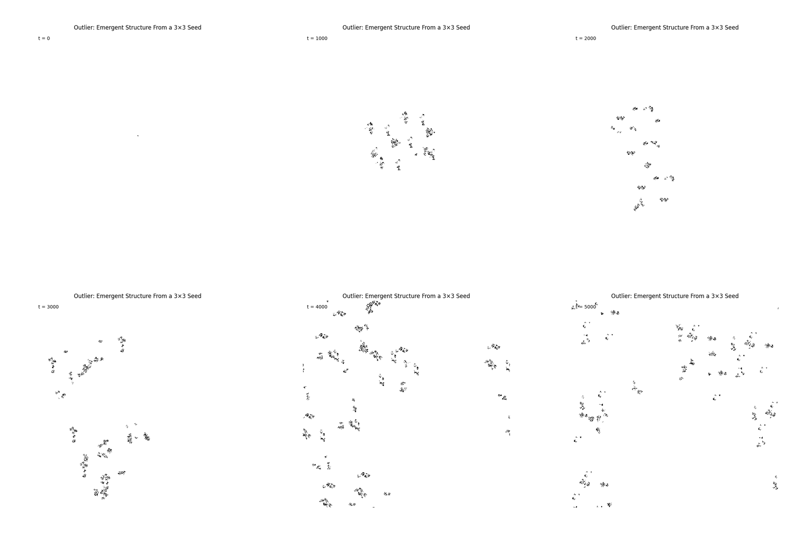
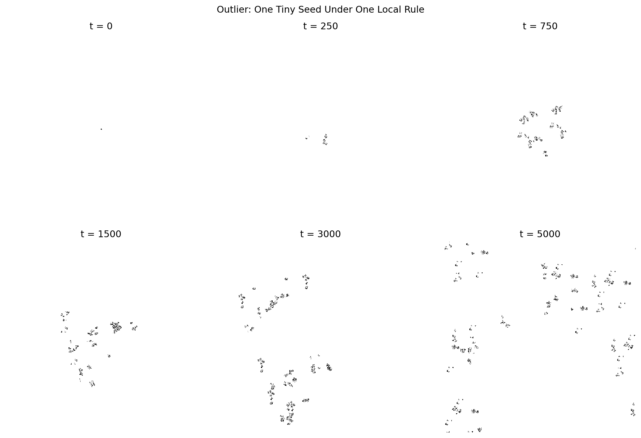
The published rule can produce rich behaviour from sparse random initial conditions.
Small shape-changing clusters appear.
Some clusters produce additional clusters.
Some periodically duplicate.
Multiple smaller structures can assemble into larger formations.
Those formations can themselves replicate.
Collections of them can eventually form the boundary of a still larger expanding complex.[5]
So the published system contains organization at multiple scales:
cells
  ↓
clusters
  ↓
replicating formations
  ↓
larger expanding complex
Replication appears at more than one scale.
That is already strange.
But we have spent enough of this book learning not to stop at strange.
There Was Still a Problem
Suppose we see:
A
and later:
A A
It is tempting to say:
A reproduced.
But perhaps the first A did not cause the second one.
Perhaps the local dynamics simply created another similar-looking configuration nearby.
Those are completely different claims.
visual recurrence
≠
causal reproduction
So in 2026, Arend Hintze and Clifford Bohm returned to Outlier with a much stronger question.
They reconstructed causal ancestry.[6]
Who Caused Whom?
The method asks something close to:
Which cells in the previous state were necessary for this later cell to appear?
At cell level:
previous cells
     ↓
causal contribution
     ↓
new cell
Those dependencies can then be aggregated into relationships between larger structures:
cluster A
    ↓
cluster B
    ↓
cluster C
Now the question is no longer merely:
does this look like that?
It becomes:
did this organization
causally contribute to
the existence of that organization?
That gives us an ancestry graph.
The 2026 analysis found branching causal reproduction in Outlier: earlier structures could causally produce multiple later structures, which could themselves participate in continuing lineages.[6]
That is a substantially stronger claim than visual similarity.
    flowchart TD
    subgraph Visual
        V1["Pattern at t"] -. "looks similar to" .-> V2["Pattern at t+1"]
    end

    subgraph Causal
        C1["Cells at t"] -->|"necessary contribution"| C2["Cells at t+1"]
        C2 --> C3["Aggregate causal relationships"]
        C3 --> C4["Earlier structure causally contributes to later structure"]
    end
The distinction will matter enormously in the next chapter.
433 Copies
The 2026 experiment used a much larger system than the small examples we will run later.
It ran Outlier on:
grid       1024 × 1024
boundary   periodic
duration   20,000 updates
The resulting causal analysis contained tens of millions of cluster instances and causal relationships.[6]
Consider the original seed cluster, called c0.
Within the first 10,000 updates, the researchers identified:
433
copies causally descending from that original seed.[6]
But those descendants did not indefinitely continue the same c0 lineage.
So we immediately learn something useful:
replication
≠
successful long-term lineage
Producing another instance is not the same as founding a persistent dynasty.
Then They Found Better Replicators
Other structures generated branching, multi-generation causal lineages.
One cluster type, c2, became particularly useful for tracing reproduction through the causal graph.[6]
The surrounding environment also mattered.
Replicators produced:
debris
collisions
fragments
recombinations
and some later replicating structures arose through those interactions.
So the system is not simply doing:
copy parent
It is closer to:
replicating process
        ↓
interaction
        ↓
fragments
        ↓
collisions
        ↓
recombination
        ↓
new structures
That is much more interesting than simple geometric copying.
But we should still be careful about what words we attach to it.
A Replicator May Not Be Connected
One of the most provocative findings from the causal analysis is that a self-replicating organization does not necessarily have to correspond to one compact connected cluster.
Some causally reproducing structures consisted of multiple spatially separated components whose combined causal dynamics participated in reproduction.[6]
The authors describe this in terms of distributed, multi-component selfhood.
For this book, we will keep the narrower result.
Causal self-replication can be distributed across multiple spatial components.
That does not yet establish that those components constitute one natural individual.
Those are different claims.
A system like:
     A
    / \
   B   C
    \ /
     D
might form one causally reproducing organization even though its visible components are spatially separated.
So connected geometry is not sufficient as a universal definition of a replicator.
But we should not jump from:
distributed causal reproduction
to:
one distributed individual
without another experiment.
That distinction is exactly the kind of thing this book is supposed to preserve.
This Is Why Outlier Is Useful to Us
Outlier has an unusually useful combination of properties.
Its underlying world is:
binary
local
deterministic
spatial
small-rule
reproducible
Yet the published experiments report:
emergent structures
hierarchical organization
causal self-replication
multiple generations
interaction
recombination
multi-component reproduction
The 2026 authors argue for a stronger interpretation involving distributed selfhood.[6]
We are not required to adopt that interpretation.
What matters to us is that causal analysis lets us separate several questions that animations otherwise collapse together:
Did another pattern appear?

Was it similar?

Did the earlier structure cause it?

Did a lineage continue?

Were several components jointly necessary?

Does that causal organization deserve to be called one individual?
Those are six different questions.
That makes Outlier an extraordinary reference system for our method.
But Outlier Is Not Life
Nothing above establishes that Outlier is alive.
We have not established:
learning
understanding
self-maintenance
general-purpose adaptation
deliberate self-modification
knowledge assimilation
knowledge transfer
cumulative capability acquisition
open-ended functional improvement
Nor does causal self-replication automatically establish any of those things.
The supported result is narrower:
Very simple digital physics can support emergent structures for which causal analysis identifies genuine, branching and sometimes multi-component self-replication.
That is already remarkable.
It does not need embellishment.
What About Flow-Lenia?
It is tempting to choose Flow-Lenia as our main reference system instead.
Visually, Flow-Lenia is much closer to what we intuitively imagine as an organism.
Its mass-conserving continuous dynamics can produce localized structures with complicated behaviour, and parameters governing those structures can themselves become localized within the simulated world. This permits multiple kinds of patterns to coexist and interact under locally different dynamics.[2]
Researchers have also measured evolutionary activity in Flow-Lenia.[2]
For studying:
continuous morphology
movement
mass flow
localized parameters
multispecies interactions
Flow-Lenia may be the richer substrate.
But Outlier has an enormous advantage for what we want to do next.
We can almost completely expose its mechanism.
There are only:
two cell states
512 neighborhood cases
one deterministic transition table
No neural network.
No hidden controller.
No floating-point organism representation.
That makes it an unusually good object to reproduce and attack.
Let’s Implement It
The exact rule is published.
The Outlier paper provides the complete 512-entry rule encoded as a standard MAP string.[5]
It also provides a tiny 3 × 3 seed that reproduces the published seed dynamics.
The rule is:
ERETQB4eHWkQ7xD4eYZosBQZFixOBHmtFeehExrKVhURLRAqGxeIlSO1JYZP6DRi69rop7TQCkvWTIag7kAS8g
The seed is:
.1.
111
..1
That is enough to begin.
Decode the Rule
A Moore neighborhood has nine cells.
We assign them these binary weights:
256 128  64
 32  16   8
  4   2   1
A binary 3 × 3 neighborhood therefore maps to an integer from 0 through 511.
For example:
1 0 0
0 1 0
0 0 1
becomes:
256 + 16 + 1 = 273
The corresponding entry in the 512-entry transition table determines the next state of the center cell.
The published MAP string contains those rule bits encoded in Base64.
import base64
import numpy as np


OUTLIER_MAP = (
    "ERETQB4eHWkQ7xD4eYZosBQZFixOBHmtFeehExrKVhURLRAq"
    "GxeIlSO1JYZP6DRi69rop7TQCkvWTIag7kAS8g"
)


def decode_map_rule(encoded: str) -> np.ndarray:
    """Decode the published 512-bit MAP rule."""
    padding = "=" * ((4 - len(encoded) % 4) % 4)
    raw = base64.b64decode(encoded + padding)

    bits = np.unpackbits(
        np.frombuffer(raw, dtype=np.uint8)
    )

    if len(bits) < 512:
        raise ValueError(
            "MAP rule contains fewer than 512 bits"
        )

    return bits[:512].astype(np.uint8)


RULE = decode_map_rule(OUTLIER_MAP)
At this point it is tempting to continue.
We should not.
Everything that follows depends on us having decoded the correct universe.
So before we trust the simulation, we test the decoder.
Verify Before We Trust It
The paper gives us two properties we can check immediately.
The rule should contain:
512 outputs
220 live outputs
So:
assert RULE.shape == (512,)
assert int(RULE.sum()) == 220
If either assertion fails, we stop.
But we can do better.
The published rule is rotationally symmetric.[5]
That means rotating a neighborhood through a quarter turn must not change the corresponding rule output.
We can test every possible neighborhood.
def index_to_grid(index: int) -> np.ndarray:
    bits = np.array(
        [
            (index >> shift) & 1
            for shift in range(8, -1, -1)
        ],
        dtype=np.uint8,
    )
    return bits.reshape(3, 3)


def grid_to_index(grid: np.ndarray) -> int:
    value = 0

    for bit in grid.reshape(-1):
        value = (value << 1) | int(bit)

    return value


def verify_rotational_symmetry(
    rule: np.ndarray,
) -> None:
    for index in range(512):
        grid = index_to_grid(index)
        expected = int(rule[index])

        rotated = grid.copy()

        for _ in range(3):
            rotated = np.rot90(rotated)

            rotated_index = grid_to_index(
                rotated
            )

            assert (
                int(rule[rotated_index])
                == expected
            ), (
                index,
                rotated_index,
                expected,
                int(rule[rotated_index]),
            )


verify_rotational_symmetry(RULE)
If that completes successfully, we have checked:
decoded entries             512
live outputs                220
quarter-turn symmetry       all 512 neighborhoods
This is a tiny piece of verification.
It is also load-bearing.
If our MAP decoder or bit ordering is wrong, every later experiment would be about a different cellular automaton.
The visual output might still look fascinating.
It would simply be irrelevant.
One Update
Now we can implement one step of the universe.
def outlier_step(
    state: np.ndarray,
    rule: np.ndarray,
) -> np.ndarray:

    nw = np.roll(
        np.roll(state, 1, axis=0),
        1,
        axis=1,
    )

    north = np.roll(state, 1, axis=0)

    ne = np.roll(
        np.roll(state, 1, axis=0),
        -1,
        axis=1,
    )

    west = np.roll(state, 1, axis=1)

    centre = state

    east = np.roll(state, -1, axis=1)

    sw = np.roll(
        np.roll(state, -1, axis=0),
        1,
        axis=1,
    )

    south = np.roll(state, -1, axis=0)

    se = np.roll(
        np.roll(state, -1, axis=0),
        -1,
        axis=1,
    )

    neighborhood = (
          (nw.astype(np.uint16) << 8)
        | (north.astype(np.uint16) << 7)
        | (ne.astype(np.uint16) << 6)
        | (west.astype(np.uint16) << 5)
        | (centre.astype(np.uint16) << 4)
        | (east.astype(np.uint16) << 3)
        | (sw.astype(np.uint16) << 2)
        | (south.astype(np.uint16) << 1)
        |  se.astype(np.uint16)
    )

    return rule[neighborhood]
Look at what is missing.
There is no:
replicate()
No:
organism()
No:
find_child()
No:
evolve()
Only the transition rule.
Add the Published Seed
The seed is:
SEED = np.array(
    [
        [0, 1, 0],
        [1, 1, 1],
        [0, 0, 1],
    ],
    dtype=np.uint8,
)
Place it in the center of a periodic world.
def make_world(
    size: int = 512,
) -> np.ndarray:

    world = np.zeros(
        (size, size),
        dtype=np.uint8,
    )

    row = size // 2 - 1
    col = size // 2 - 1

    world[
        row:row + 3,
        col:col + 3,
    ] = SEED

    return world
And run:
RULE = decode_map_rule(OUTLIER_MAP)

assert RULE.shape == (512,)
assert int(RULE.sum()) == 220

verify_rotational_symmetry(RULE)

world = make_world(512)

for tick in range(5000):
    world = outlier_step(
        world,
        RULE,
    )

    if tick % 100 == 0:
        print(
            tick,
            int(world.sum()),
        )
That gives us a compact implementation of the published local physics.
But there is an important distinction we must make before interpreting anything it produces.
Our Implementation Is Not Yet the Full Published Experiment
The code above reproduces:
the published transition rule
+
the published seed
+
periodic local dynamics
That does not mean every experiment we run is equivalent to the published experiments.
The 2026 causal study used:
grid       1024 × 1024
boundary   periodic
duration   20,000 updates
Our teaching implementation may use smaller worlds or shorter runs.
That difference is not cosmetic.
The earlier Outlier work reports a strong scale effect: sparse random worlds smaller than roughly 512 × 512 did not produce the larger replicating formations seen in the principal experiments.[5]
So we establish a rule now:
A result obtained from a smaller or shorter Outlier run is a result about that run. It must not automatically be generalized to the full published Outlier regime.
This becomes particularly important in the next chapter.
If we run:
512 × 512
for
1,600 generations
then our claims apply to:
the structures observable
in that 512 × 512
1,600-generation experiment
They do not automatically apply to:
1024 × 1024
20,000-generation
hierarchical Outlier dynamics
Scale is part of the experimental condition.
Something Important Has Already Changed
Remember our crystal from Chapter 11.
It grew because we explicitly chose a growth rule.
Outlier is different.
We did not define:
parent
offspring
family
replicator
formation
inside its transition law.
Those are descriptions applied after larger organizations appeared.
That makes Outlier useful for a very particular purpose.
It allows us to ask:
When does our interpretation outrun the mechanism?
That is exactly what the next chapter will test.
What We Should Steal
Outlier gives us several ideas worth carrying forward.
1. Do not design the organism
We can design or discover local physics and allow candidate structures to arise within it.
2. Do not assume one scale
Interesting organization may exist simultaneously at:
cell
cluster
formation
larger structure
without one scale automatically being privileged.
3. Do not equate connected geometry with causal organization
A causally reproducing structure may involve spatially separated components.
That does not establish individuality.
It tells us only that connectedness is not enough.
4. Track causation
Visual resemblance is not sufficient evidence for:
reproduction
inheritance
influence
ancestry
Whenever possible, reconstruct the dependencies.
5. Let interactions matter
Collision, recombination and environmental interference can generate novelty without us injecting a mutation operator from outside.
Those are useful lessons.
They are not a specification for our next system.
What We Should Not Steal Yet
Outlier also tempts us into vocabulary we have not earned.
Words such as:
organism
individual
family
offspring
self
collective
flocking
are extremely seductive once an animation starts moving.
So we are not going to carry those words forward unquestioned.
In particular, causal ancestry creates an obvious hypothesis:
Structures that share recent causal ancestry may behave as one continuing organization.
Perhaps.
But perhaps what looks like family behaviour is merely:
spatial proximity
shared local flow
common environmental disturbance
Perhaps connected clusters are the wrong units.
Perhaps causal families are the wrong units.
Perhaps there is no unique natural unit at all.
Those are experimental questions.
Outlier Is a Reference Case, Not Our Destination
Outlier does not know anything about:
the internet
external knowledge
its own rule
experiments
checkpoints
forking
merging
deliberate modification
But that is not a criticism.
Those capabilities are irrelevant to what Outlier has already demonstrated.
For us, Outlier establishes a lower reference point:
How much complicated causal organization can appear before anything resembling intelligence is required?
That is enormously useful.
But we are not going to take Outlier and start bolting capabilities onto it.
That would simply create another cargo cult.
Instead:
OUTLIER
↓
observe
↓
form interpretation
↓
attack interpretation
↓
keep only what survives
↓
return to our controlled laboratory
That is the bridge to the rest of the book.
Evidence Ledger
At this point we can separate what is established from what remains open.
| Claim | Status | Evidence |
|---|---|---|
| The published MAP decodes to 512 binary outputs | SUPPORTED | exhaustive decode |
| The decoded rule contains 220 live outputs | SUPPORTED | direct count |
| The decoded rule is invariant under quarter-turn rotations | SUPPORTED | exhaustive 512-neighborhood test |
| Outlier produces self-replicating organization under published experimental conditions | SUPPORTED FROM PUBLISHED WORK | Yang 2025 |
| Causal ancestry identifies genuine branching replication | SUPPORTED FROM PUBLISHED WORK | Hintze & Bohm 2026 |
| Causal reproduction can span multiple spatial components | SUPPORTED FROM PUBLISHED WORK | Hintze & Bohm 2026 |
| Multi-component reproduction establishes one natural individual | UNTESTED HERE | requires an additional criterion |
| Shared ancestry causes coordinated motion | UNTESTED HERE | next chapter |
| Our smaller teaching run reproduces the entire published Outlier regime | NOT CLAIMED | scale and duration differ |
| Outlier is alive | NOT CLAIMED | evidence insufficient |
This ledger matters.
The most interesting entries may eventually be the ones that fail.
What Is the Closest Thing We Have?
So is Outlier digital life?
We will not make that claim.
A narrower statement survives:
Outlier is a striking demonstration that extremely compact digital physics can support emergent, hierarchical self-replication, and that causal reconstruction can identify reproduction distributed across multiple spatial components.
The entire local universe is specified by:
512 bits of transition law
+
initial state
+
space
+
time
From that, unexpectedly complicated causal organization can appear.
But the animation gives us more interpretations than the evidence has earned.
So before returning to our own Digital Crystal, we are going to do something more important.
We are going to attack Outlier.
We will ask:
Is recurrence really reproduction?

Can we reconstruct causal descendants?

Does shared ancestry predict shared behaviour?

Does the apparent family effect survive
a better control?

What happens when proximity is separated
from ancestry?

And what can our finite replication
actually tell us about the larger system?
Outlier is not the organism from which our later Digital Crystal descends.
It is the hostile reference case that teaches us which interpretations survive.
We are not going to copy it.
We are going to try to prove ourselves wrong about it.
Next:
Is It Really Reproducing?
References
[1] Sayama, H. & Nehaniv, C. L. Self-Reproduction and Evolution in Cellular Automata: 25 Years After Evoloops. Artificial Life 31(1), 81–95 (2025).
[2] Plantec, E., Hamon, G., Etcheverry, M., Chan, B. W-C., Oudeyer, P-Y. & Moulin-Frier, C. Flow-Lenia: Emergent Evolutionary Dynamics in Mass Conservative Continuous Cellular Automata. Artificial Life 31(2), 228–250 (2025). doi:10.1162/artl_a_00471
[3] Packard, N. H. & McCaskill, J. S. Open-Endedness in Genelife. Artificial Life 30(3), 356–389 (2024). doi:10.1162/artl_a_00426
[4] Agüera y Arcas, B. et al. Computational Life: How Well-formed, Self-replicating Programs Emerge from Simple Interaction. arXiv:2406.19108 (2024).
[5] Yang, B. Emergence of Self-Replicating Hierarchical Structures in a Binary Cellular Automaton. Artificial Life 31(1), 96–105 (2025). doi:10.1162/artl_a_00449
[6] Hintze, A. & Bohm, C. Rethinking self-replication: detecting distributed selfhood in the Outlier cellular automaton. npj Complexity 3, 11 (2026).
