13: Is It Really Reproducing?
Something strange happened while we were looking at Outlier.
We had started with a question about reproduction.
Then I watched the simulation.
And I thought:
That looks like flocking.
That is exactly the kind of observation that can get us into trouble.
Humans are extraordinarily good at seeing things in motion and assigning meaning to them.
We see:
a shape
another shape
movement
coordination
and very quickly turn that into:
organisms
offspring
groups
flocks
But this book has one rule that matters more than almost any other:
appearance
is not
evidence
So instead of calling it flocking, we stopped.
And measured it.
That led us into a much deeper investigation than I expected.
The Problem With Watching Artificial Life
Here is the Outlier simulation again.
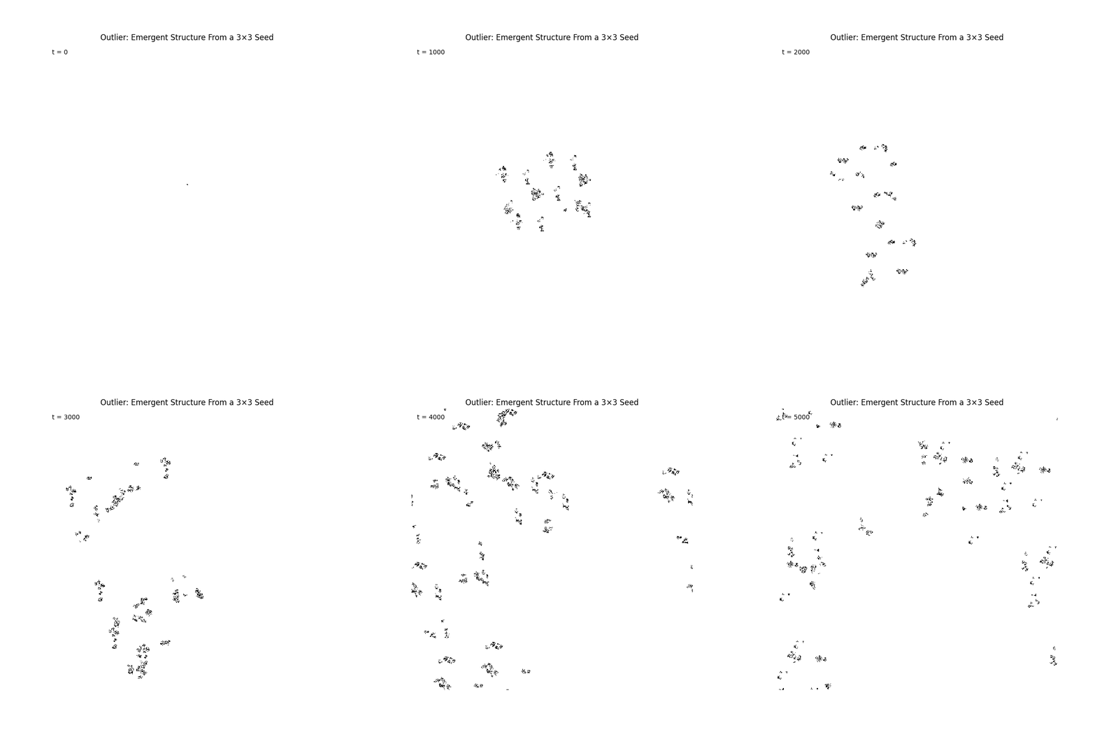
The published Outlier cellular automaton running from its small initial seed.
It is very difficult to watch something like this without inventing nouns.
You start saying:
that thing moved
that thing split
those things are travelling together
that one produced another one
But every noun contains a hypothesis.
What is a thing? What counts as the same structure at a later time? What makes one structure the parent of another? What makes two nearby structures part of the same causal process rather than merely close together?
These are not philosophical decorations.
They are experimental questions.
First Question: Is It Really Reproducing?
In the previous chapter we introduced Outlier because it gives us something unusually valuable.
It is extremely simple at the substrate level.
The world is a binary cellular automaton.
Each cell sees a 3 × 3 neighborhood.
That neighborhood gives us one of 512 possible local configurations.
A fixed rule determines whether the centre cell will be alive or dead on the next step.
There is no class called Organism.
There is no method called reproduce().
There is no explicit genome object.
And yet large structures appear.
Some structures recur.
Some appear to produce more structures.
That makes Outlier ideal for our purposes.
If reproduction occurs here, it cannot be because the programmer wrote:
if organism.ready:
    organism.reproduce()
Something more interesting must be happening.
Similarity Is Not Reproduction
Suppose we see this:
time t

    A

time t + 500

    A     A
It is tempting to say:
A reproduced.
But that observation alone does not establish reproduction.
Perhaps both copies were produced independently by the surrounding environment.
Perhaps the second structure would have appeared even if the first one had never existed.
Perhaps what we are calling two structures are actually parts of a larger repeating process.
So reproduction is not merely a question of similarity.
It is a causal claim.
We want something closer to:
parent existed
↓
parent participated causally in a process
↓
later candidate appeared
↓
without the relevant earlier structure,
the later structure would not have appeared in the same way
That is a much stronger statement.
Counterfactual Causality
Because Outlier is a cellular automaton, we have an unusually clean opportunity.
For every live cell at time t + 1, we know exactly which 3 × 3 neighborhood produced it.
So we can ask:
Which live cells in the preceding neighborhood were actually necessary for this cell to become alive?
Our simplified test works like this.
Take a live child cell.
Then, one at a time, remove each live predecessor from its local neighborhood.
Re-evaluate the cellular automaton rule.
If removing a predecessor changes the child from alive to dead, then that predecessor was positively necessary under this counterfactual test.
    flowchart TD
    A["Child cell is alive"] --> B["Identify live predecessors in 3×3 neighborhood"]
    B --> C["Remove one predecessor at a time"]
    C --> D["Recompute rule on modified neighborhood"]
    D --> E{"Child becomes dead?"}
    E -- Yes --> F["Record causal dependency: predecessor → child"]
    E -- No --> G["Predecessor not necessary"]
This is not a complete theory of causality.
But it gives us something much stronger than visual resemblance.
It gives us a causal graph.
From Cells to Structures
Cell-level causality produces a huge amount of information.
So we aggregate cells into connected clusters.
Then causal dependencies between cells become causal relationships between clusters.
The result looks approximately like:
cluster at t
     ↓
cluster at t+1
     ↓
cluster at t+2
     ↓
...
with branching where one earlier organization contributes to multiple later structures.
For our 512 × 512 experiment over 1,600 generations we found:
138,891 clusters
196,466 causal edges
That is already a useful warning.
The visual animation looks as though it contains a collection of fairly obvious moving objects.
The causal graph tells us that underneath that appearance is a very large network of dependencies.
Scope of This Experiment
Before going further, we need to pin down exactly what this chapter can and cannot establish.
Our run is:
grid          512 × 512
generations   1,600
boundary      periodic
The published causal Outlier study used a substantially larger regime:
grid          1024 × 1024
updates       20,000
boundary      periodic
That difference matters.
Outlier is scale-sensitive.
Larger and later hierarchical formations may not be represented in a shorter 512 × 512 run.
So every result in this chapter should be read as:
a result about the structures observable in our 512 × 512, 1,600-generation reproduction of Outlier.
We must not automatically generalize a null result here to the larger published regime.
This limitation will matter again near the end of the chapter.
Finding c2 Again
The published Outlier seed starts as a tiny configuration:
.1.
111
..1
After two updates it produces a small structure we call c2.
In our simulation that structure had:
area          6
bounding box  3 × 3
Instead of searching for arbitrary repeating shapes, we derived the actual c2 signature directly from the known initial seed.
Then we searched the entire run for later occurrences of that structure, allowing translation and rotation.
We found:
144 c2 occurrences
between:
t = 2
and
t = 1598
But recurrence still does not prove reproduction.
So we combined recurrence with the causal graph.
A Causal Family Tree
For every c2, we searched forward through the causal graph for later c2 structures reachable through that causal history.
The original c2 at t = 2 produced a branching causal structure with four later c2 descendants.
The complete return graph contained:
99 visible c2 return edges
The full graph was too complicated to use as an illustration, so the figure shows a deliberately pruned family.
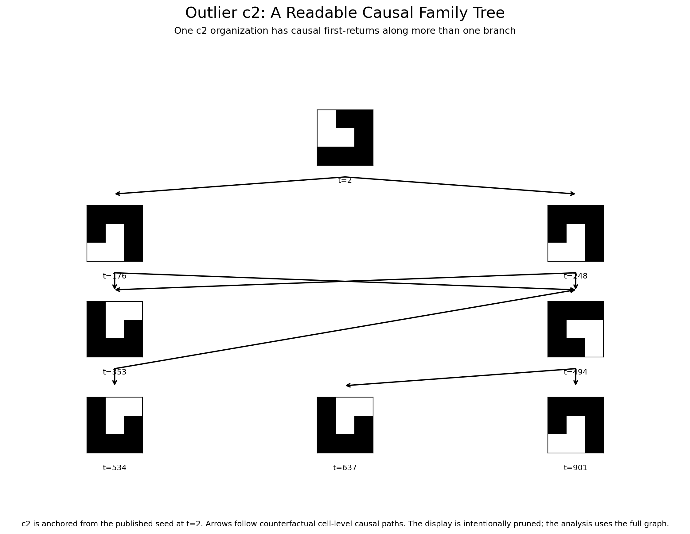
A readable subset of the Outlier c2 causal family tree. The visual is pruned; the analysis uses the full causal graph.
This is much stronger evidence than:
I saw one shape and later saw several similar shapes.
We can now say something closer to:
Later occurrences of the c2 structure are reachable through measurable causal ancestry originating in earlier c2 structures.
That is the kind of evidence we need before using words such as reproduction.
Causal Reproduction Survives in This Run
Within our 512 × 512, 1,600-generation reproduction, the evidence for c2 reproduction is not merely geometric recurrence.
It is:
structural recurrence
+
counterfactual causal ancestry
+
branching lineage
That distinction matters.
So the narrow claim survives:
In our run, recurring c2 structures participate in a branching causal return graph.
That does not establish life.
It does not establish a natural individual.
It does establish something much stronger than visual copying.
Then I Saw the Flock
While looking at the same simulation, another visual pattern became difficult to ignore.
Groups of structures appeared to move together.
Not merely outward.
Together.
It looked remarkably like flocking.
But we had just spent several chapters warning ourselves against doing exactly this.
So we made the visual impression into a hypothesis.
What Would Flocking Mean?
We did not begin by trying to reproduce every formal definition from swarm biology or active-matter physics.
We started with a much narrower question:
Do nearby persistent moving structures travel in unusually similar directions?
That can be measured.
First we needed persistent motion tracks.
Using the causal graph, we followed plausible continuations of clusters through time.
The run produced:
13,635 persistent motion tracks
with minimum length:
8 generations
Across those tracks we obtained:
633,808 motion observations
Each observation gave us:
position
velocity
time
causal identity
That was enough to perform a first test.
Measuring Directional Alignment
For two velocity vectors (v_i) and (v_j), we normalize them and take their dot product:
+1  = same direction
 0  = no directional agreement
-1  = opposite directions
Then we compare simultaneously moving structures at different spatial separations.
For performance, we do not compare every structure with every other structure.
We use a spatial index and examine nearby pairs.
That is also a better experiment.
Structures on opposite sides of the universe are not particularly useful for measuring local collective motion.
The First Result
The first experiment produced a striking result.
At short distances, observed velocity alignment was approximately:
0.74
while a velocity-shuffled control was much lower.
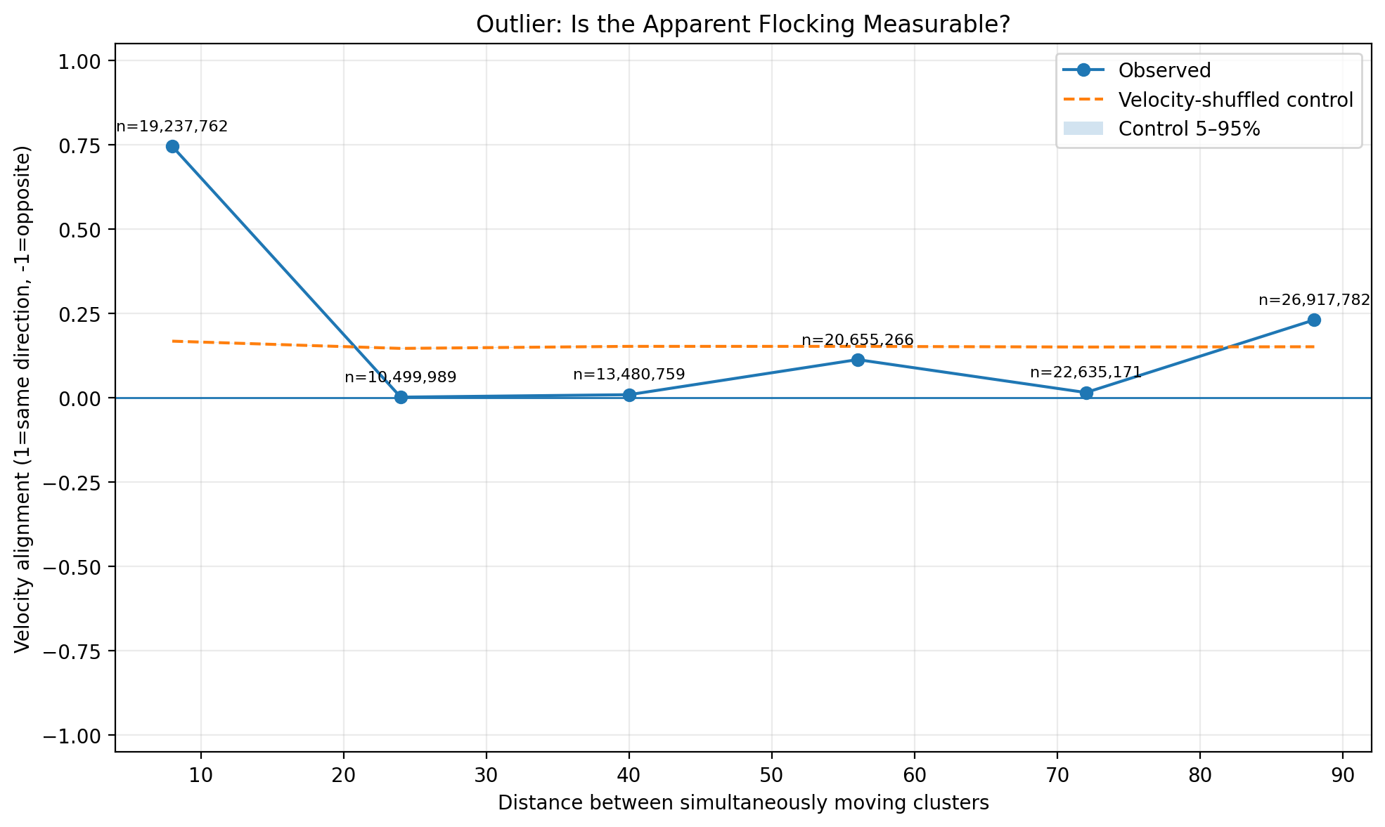
Nearby persistent structures exhibit much stronger directional alignment than a shuffled velocity control.
So the visual observation was not completely imaginary.
There really was measurable short-range motion coherence.
But this still did not prove flocking.
We had immediately created another problem.
Maybe Everything Is Simply Moving Outward
Outlier develops as an expanding structure.
Suppose nearby clusters sit on the same expanding front.
They might move in similar directions simply because both are being carried outward.
Imagine two pieces of debris on the same expanding circular wave.
They could have very similar velocity vectors without interacting with one another at all.
So we needed another control.
Removing Radial Expansion
For each position (x_i), we calculate its radial direction relative to the centre:
radial motion
+
non-radial motion
and remove the radial component.
If the apparent flocking was really just expansion, the alignment should collapse.
Instead we found:
raw short-range alignment        = 0.7373
radial-subtracted alignment      = 0.7427
shuffled residual control        = 0.1933
The alignment did not disappear.
It barely changed.
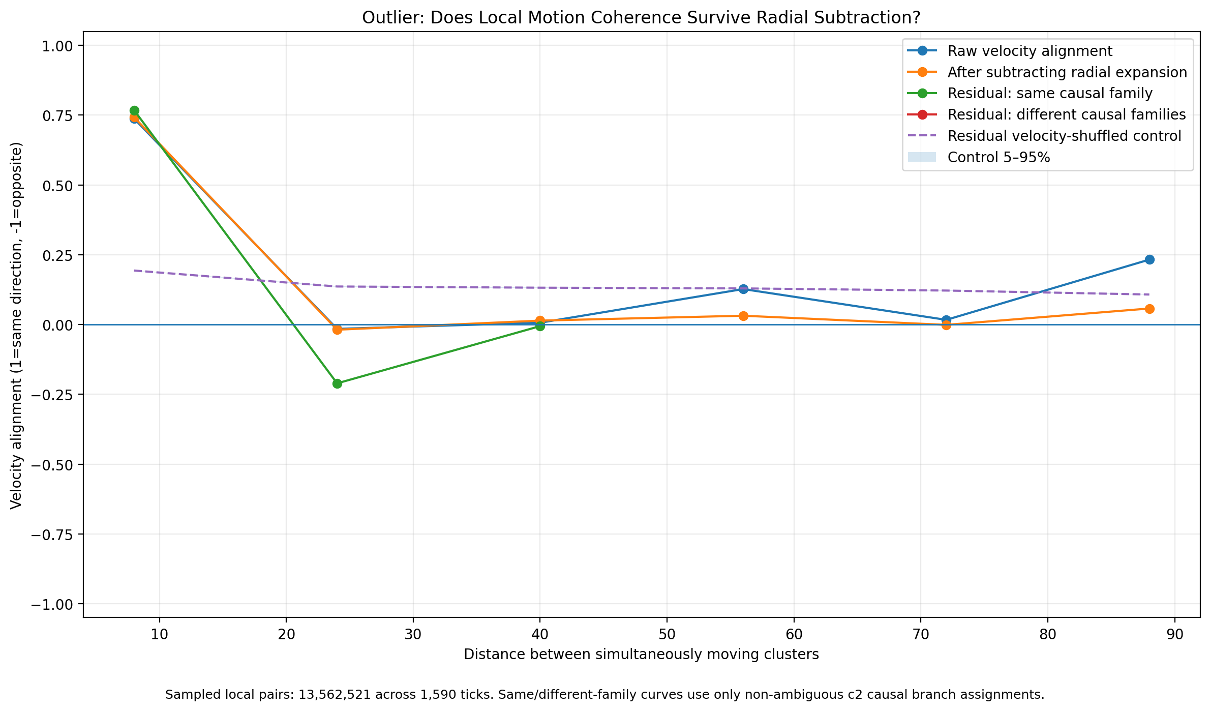
Short-range motion coherence survives subtraction of the global radial expansion field.
So we could rule out one simple explanation:
The observed coherence is not explained merely by every structure moving radially away from the original seed.
That made the result more interesting.
And then the causal analysis gave us another possibility.
Shared Causal History
Several spatially disconnected clusters can participate in the same causal organization.
So what looks like:
thing A
thing B
thing C
might actually be:
component A
component B
component C
        ↓
one distributed causal process
That does not establish that the components form one natural individual.
It gives us a narrower hypothesis:
Does shared causal organization explain the apparent coordinated motion?
So we asked:
Do structures belonging to the same causal lineage move more coherently?
Giving Structures Causal Families
Our first family definition was too narrow.
It started with four branches descending from one early c2.
That produced strong same-family alignment:
0.768
but no useful different-family comparison.
So we strengthened the definition.
Every cluster was assigned its most recent identifiable c2 ancestor.
If a cluster itself was c2, it began a new family.
Otherwise we propagated ancestry through the causal graph.
If equally close causal paths disagreed, we marked the assignment ambiguous rather than inventing an answer.
The coverage was remarkable.
Among:
138,891 clusters
we assigned a recent c2 ancestor to:
138,132
Only:
10 ambiguous
749 unassigned
Among our motion observations:
633,696 / 633,808
received a recent-c2 family label.
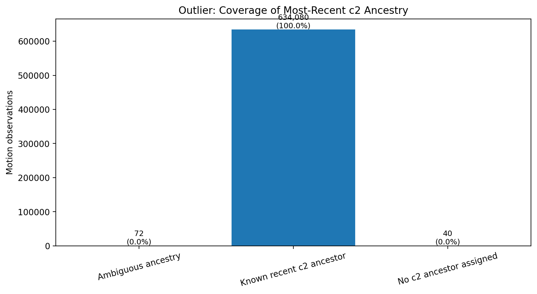
Almost every tracked moving structure in this single-seed experiment can be associated with a recent c2 causal ancestor.
That tells us something important about this experiment.
Almost everything we are tracking belongs to a branching causal history.
But causal history alone does not tell us whether that history explains current motion.
A Very Exciting Result
When we compared nearby structures after subtracting a local background flow, we initially found:
same recent-c2 family         = 0.828
different recent-c2 family    = -0.349
That looked spectacular.
Perhaps causal relatives really were moving together.
Perhaps different families were even moving against one another.
But there was a problem.
The control itself could create the negative result.
Our Experiment Was Wrong
This is worth slowing down for.
To estimate the local environmental flow around object A, we averaged nearby velocity vectors after excluding structures from A’s own family.
When comparing two different families A and B, B could therefore contribute to the estimate of A’s background — and A could contribute to the estimate of B’s background.
In the simplest case:
So the -0.349 result was not trustworthy.
    flowchart TD
    A["Object A velocity"] --> B["Background estimate for A uses B velocity"]
    B --> C["Residual A ≈ vA - vB"]
    D["Object B velocity"] --> E["Background estimate for B uses A velocity"]
    E --> F["Residual B ≈ vB - vA"]
    C --> G["Residuals artificially anti-correlated"]
    F --> G
This is exactly why experiments need controls.
And why controls themselves need criticism.
Pair-Excluded Background Flow
We fixed the problem.
When testing a pair from families α and β, we estimated local background motion while excluding both families from both estimates.
Now neither member of the tested pair could create the other’s residual.
Using this stronger control we obtained:
Same recent c2 ancestor          0.746
Very close c2 ancestry           0.101
Close c2 ancestry                0.032
Distant c2 ancestry              0.135
Very distant c2 ancestry         0.081
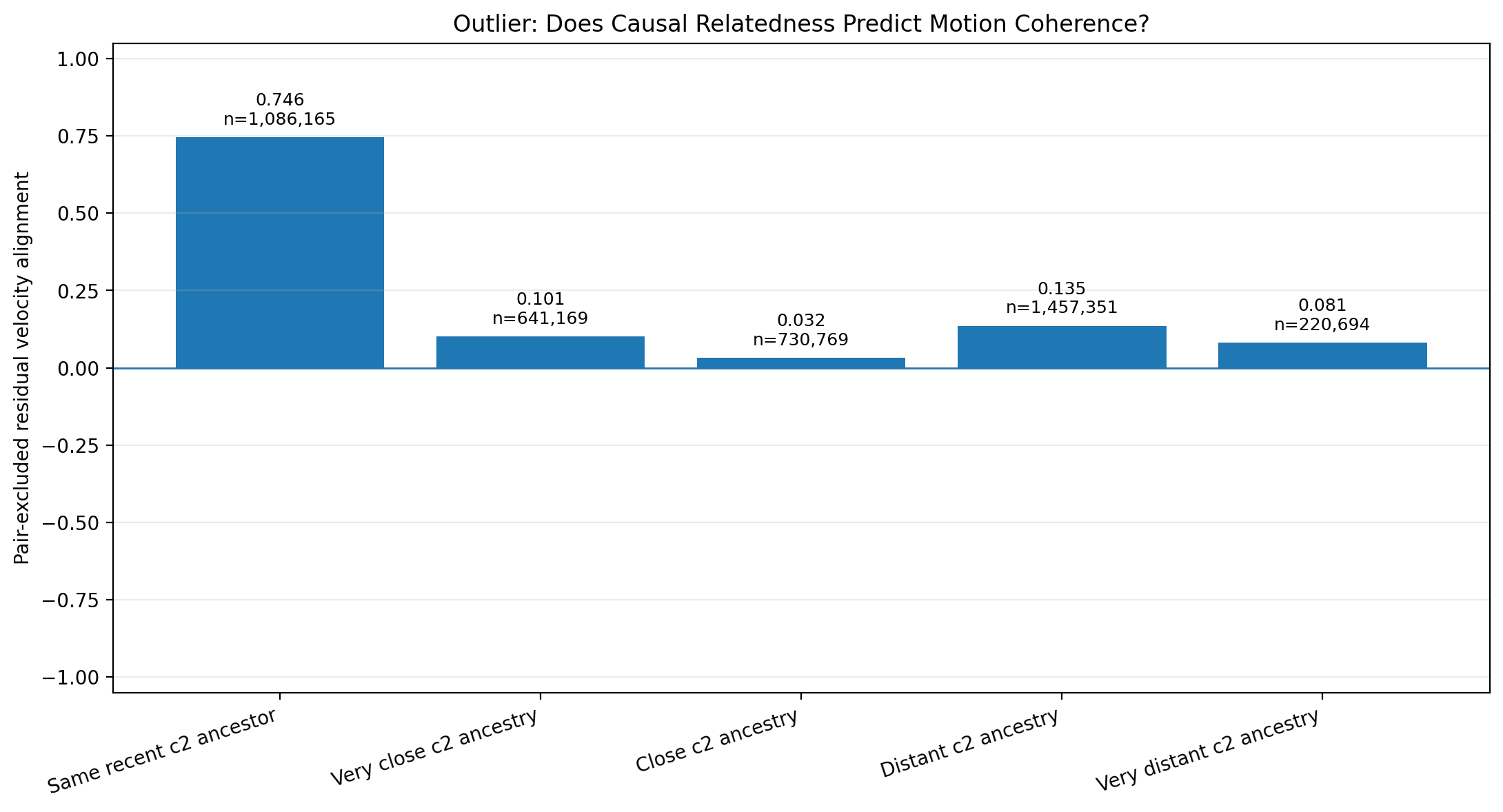
Motion coherence is extremely high for structures sharing the same recent c2 ancestor, while more distant genealogical relationships show much weaker coherence.
This again looked spectacular.
The apparent gap between:
same recent c2 ancestor    0.746
very close ancestry        0.101
was:
0.645
That looked like strong evidence that recent causal ancestry predicted dynamical organization.
But there was another problem.
The Four-and-a-Half-Cell Problem
The structures sharing the same recent c2 ancestor were also extremely close together.
Their mean separation was only about:
4.5 cells
Other causal groups were typically tens of cells apart.
So we had confounded:
causal relatedness
with:
spatial proximity
Perhaps structures sharing a family move together because they are parts of the same tiny local formation.
Perhaps any two structures that close together would show similar motion.
Once again, the exciting interpretation had outrun the evidence.
So we performed another experiment.
Distance-Matched Causal Coherence
We constructed a matched dataset.
For a same-family pair, we searched for different-family comparisons occurring under approximately the same conditions.
We matched on:
simulation time
spatial distance
local density
and continued to use the stronger pair-excluded background-flow correction.
The question was now very precise:
At similar times, at similar distances, and in similar local environments, do members of the same c2 causal family move more coherently than members of different families?
The underlying pair dataset contained:
2,617,077 usable pair records
The original matching analysis constructed approximately:
65,000 matched pairs per group
across hundreds of matched strata.
At first, the result appeared straightforward.
The Apparent Effect Collapsed
After matching distance, simulation time and local density, the same-family and different-family means became almost identical.
The earlier analysis gave approximately:
same-family         0.1515
different-family    0.1588
difference         -0.0073
The matched-stratum bootstrap interval crossed zero.
That was already strong evidence that the dramatic 0.645 apparent family gap had largely been a spatial-context effect.
But there was still one more problem.
The matched analysis itself assumed that same-family and different-family pairs were actually available for comparison across the distance range.
That assumption needed to be tested.
Common Support
Matching cannot create comparison data where none exists.
If almost all same-family pairs occur at one distance and almost all different-family pairs occur somewhere else, a global matched estimate can hide a region in which the effect is not actually identifiable.
So we preserved all:
2,617,077
pair records and measured the spatial overlap directly.
The original Chapter 13 distance bins were:
0–4
4–8
8–12
12–16
16–24
24–32
32–48
48–64
64–96
For the primary analysis we declared a simple operational support rule:
A distance bin must contain at least 100 same-family and 100 different-family raw pair records.
The largest contiguous region satisfying that condition was:
[4, 64) cells
This immediately changed the interpretation.
The shortest-distance regime:
0–4 cells
was outside the primary common-support region.
So we cannot claim that matching has identified the ancestry effect there.
That part of the experiment remains unresolved.
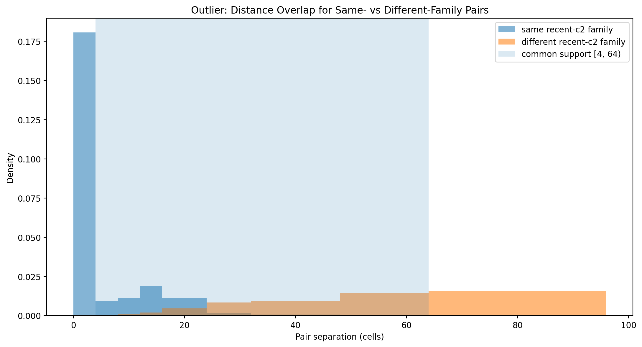
Same-family and different-family distance distributions. The shaded region marks the primary common-support interval from 4 to 64 cells.
Inside the Region We Can Actually Compare
Within the primary common-support interval:
4–64 cells
the raw descriptive data still showed an apparent family advantage:
same-family mean         0.1732
different-family mean    0.1166
raw difference          +0.0566
That is important.
Even after restricting the distance range, the unbalanced raw data still looks as though same-family pairs move more coherently.
Then we apply the original matching procedure again.
Exact matching uses:
time bin
distance bin
density bin
and takes equal numbers of same-family and different-family pairs within each matched stratum.
The result becomes:
matched same-family mean        +0.150823
matched different-family mean   +0.157890
matched pooled effect           -0.007067
Across:
64,948 matched pairs per group
659 matched strata
the equal-stratum effect was:
-0.026463
with bootstrap interval:
[-0.066450, +0.012172]
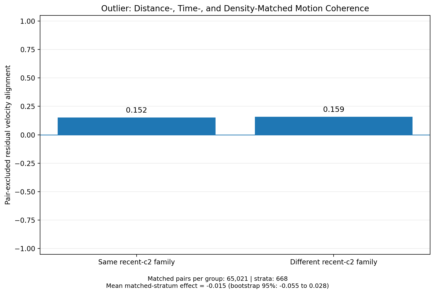
Inside the matched comparison, same-family and different-family motion coherence are essentially indistinguishable.
This is the important result.
How Much of the Original Effect Could Still Be Real?
The original apparent family gap was:
0.746 - 0.101 = 0.645
Inside common support, the upper end of the bootstrap interval is:
+0.012172
So the largest positive ancestry effect compatible with that interval is approximately:
0.012172 / 0.645
≈
1.9%
of the original apparent gap.
That gives us a much stronger statement than:
the confidence interval crosses zero.
We can now say:
Within the 4–64 cell region where the comparison has adequate empirical support, the data rule out anything remotely resembling the original apparent family effect. The upper bootstrap bound is only about 1.9% of the original 0.645 gap.
That is a real negative result.
And it is much more informative than simply saying the effect disappeared.
The Result Is Not an Artifact of One Support Threshold
The common-support criterion itself was also tested.
We repeated the analysis using minimum counts of:
50
100
250
500
same-family and different-family records per distance bin.
At threshold 50, common support expanded to:
4–96 cells
The matched pooled effect remained:
-0.0058
and the equal-stratum effect remained slightly negative:
-0.0182
At thresholds:
100
250
500
the support interval remained:
4–64 cells
and the matched result remained:
matched pooled effect     -0.0071
equal-stratum effect      -0.0265
upper bootstrap bound     +0.0122
So the conclusion does not qualitatively depend on one arbitrary minimum-count threshold.
That increases our confidence in the bounded result.
But the 0–4 Cell Regime Is Still Open
We should be equally precise about what the analysis did not resolve.
The structures sharing a recent c2 ancestor are concentrated at extremely short range.
The 0–4 cell bin lies outside the declared primary common-support region.
That means:
same-family pairs
are common there

different-family controls
are too sparse for the same comparison
So we cannot say:
ancestry has no effect at 0–4 cells.
Nor can we say:
ancestry causes the effect at 0–4 cells.
The correct status is:
UNRESOLVED
That is not a weakness in the result.
It is the correct description of what the data can identify.
So Was It Flocking?
Not on the evidence we currently have.
But the original observation was not worthless.
We learned several things.
-
Outlier exhibits strong short-range velocity coherence. That is measurable.
-
The coherence is not explained by simple global radial expansion.
-
Shared c2 ancestry initially appears to predict much stronger coherence.
-
That dramatic ancestry signal collapses after controlling spatial distance, simulation time and local density over the region where same-family and different-family pairs have adequate overlap.
-
The 0–4 cell regime remains unresolved because suitable different-family controls are too sparse there.
So the bounded claim is:
Within the 4–64 cell region where same-family and different-family pairs have adequate common support, shared recent c2 ancestry contributes no detectable additional motion coherence after matching spatial distance, simulation time and local density. The upper bootstrap bound is only about 1.9% of the original apparent 0.645 family gap. The shortest 0–4 cell regime remains unresolved.
That is not as exciting as:
We discovered flocking.
It is much better.
Because we now have some idea what the evidence actually supports.
What Might the Motion Be?
Our best current interpretation is not:
causal relatives
recognize one another
and flock
It is closer to:
local geometry
+
local cellular dynamics
+
spatial organization
↓
coherent motion
That still matters.
Remember what Outlier is.
There are no explicit moving objects.
No velocity variable.
No steering force.
No alignment rule.
No flocking controller.
At the substrate level there are only:
binary cells
local neighborhoods
one deterministic update rule
Yet from those rules emerge structures with measurable coherent local motion.
That is already remarkable.
We simply should not give that phenomenon a stronger name than our measurements justify.
## What Survived the Hypothesis?
The strongest interpretation in this chapter did not survive.
We began with:
nearby structures move coherently
↓
shared c2 ancestry may explain that coherence
Inside the region where same-family and different-family pairs can actually be compared, that explanation failed.
The matched pooled effect was approximately:
-0.0071
and the upper bootstrap bound on a positive ancestry effect was only about:
+0.0122
roughly 1.9% of the original apparent 0.645 family gap.
So the ancestry explanation does not survive over the 4–64 cell common-support interval.
But the observation that motivated it does.
### The surviving observation
Persistent moving structures exhibit strong short-range velocity coherence.
The first measurements gave approximately:
raw short-range alignment        0.7373
radial-subtracted alignment      0.7427
shuffled residual control        0.1933
Removing the global radial expansion field did not remove the effect.
So the chapter leaves us with two separate statements:
SHORT-RANGE MOTION COHERENCE
MEASURED

ANCESTRY EXPLAINS THAT COHERENCE
FAILED OVER COMMON SUPPORT
Those are not contradictory.
The experiment killed an explanation without killing the phenomenon.
### Phenomenon record
Phenomenon: Local coherent motion
Status: MEASURED
Current bounded description:
Persistent structures in this Outlier run exhibit strong short-range directional coherence that survives subtraction of the global radial expansion field.
Best current mechanistic description:
local geometry
+
local cellular dynamics
+
spatial organization
↓
coherent motion
This description does not require:
flocking
social interaction
ancestry recognition
a natural individual
### Open cross-chapter hypothesis
There is a broader possibility that should remain separate from the measured result:
Some of the local coherence may be part of a spatially propagating dynamical field rather than the motion of independent object-like structures.
For now this is only an OPEN HYPOTHESIS.
The present chapter did not measure:
phase propagation
lag versus distance
propagation velocity
dispersion relation
travelling-wave structure
So we should not call the phenomenon a wave.
A future audit can test the literal signature using the existing motion data:
activity at x,t
↓ lag
activity at x+d,t+τ
If the correlation peak moves systematically with distance, then a propagation velocity becomes measurable.
If it does not, the propagating-field interpretation should be rejected.
### Important unresolved region
The shortest-distance regime remains special.
0–4 cells
lies outside the declared common-support interval because suitable different-family controls are too sparse.
Therefore:
ANCESTRY EFFECT AT 0–4 CELLS
UNRESOLVED
We should neither promote nor dismiss it.
### What this phenomenon does not establish
This surviving motion phenomenon does not establish:
- classical flocking,
- interaction between natural individuals,
- a shared wave mechanism,
- ancestry-dependent coordination,
- organism-like units,
- or life.
It establishes something narrower and, for this project, more useful:
Simple local cellular dynamics can generate strongly coherent short-range motion even after one of the most tempting biological explanations for that motion has been removed.
That phenomenon now belongs in the project-wide phenomenon record independently of the chapter’s ancestry hypothesis.
The Most Important Result May Be Methodological
This investigation began with five words:
That looks like flocking.
If we had stopped there, we would have had a nice animation and a bad claim.
Instead:
    flowchart TD
    A["Visual impression: That looks like flocking"] --> B["Operational definition"]
    B --> C["Tracking"]
    C --> D["Velocity measurement"]
    D --> E["Shuffled control"]
    E --> F["Radial-flow control"]
    F --> G["Causal-family hypothesis"]
    G --> H["Local-flow control"]
    H --> I["Discover estimator bug"]
    I --> J["Pair-excluded control"]
    J --> K["Discover spatial confound"]
    K --> L["Distance/time/density matching"]
    L --> M["Audit common support"]
    M --> N["Bound positive effect"]
    N --> O["Keep unresolved region unresolved"]
This is exactly the process we need if we are going to talk seriously about digital life.
Interesting pictures are where questions begin.
Not where claims end.
The Database Changed How We Could Work
There was another practical lesson.
Our simulation produced:
138,891 clusters
196,466 causal edges
633,808 motion observations
2,617,077 usable pair records
Initially we recomputed expensive quantities every time we asked a new question.
That quickly became absurd.
So we created a SQLite database.
The expensive simulation became a reusable experimental specimen.
Then we improved the evidence architecture again.
The derived pair-level comparison dataset is now also preserved:
ch13_pair_datasets
ch13_pair_records
So the pipeline becomes:
    flowchart LR
    A["Outlier run"] --> B["SQLite specimen"]
    B --> C["clusters"]
    B --> D["causal edges"]
    B --> E["c2 occurrences"]
    B --> F["motion observations"]
    C & D & E & F --> G["pair-level evidence"]
    G --> H["distance matching"]
    G --> I["common-support analysis"]
    G --> J["sensitivity analysis"]
    H & I & J --> K["bounded claim"]
This matters beyond performance.
It changes how we investigate these systems.
The simulation becomes something closer to an experimental specimen.
We can ask multiple questions of the same run while preserving exactly which data each conclusion came from.
Causal Reproduction Still Survives
The flocking hypothesis weakened.
The reproduction result did not disappear with it.
We still observed:
144 c2 occurrences
and constructed causal paths between recurring c2 structures.
The original c2 at t = 2 lies at the root of a branching causal return structure.
So the evidence for reproduction is not:
it looks like one object became several
It is:
structural recurrence
+
causal ancestry
+
branching lineage
That distinction matters.
The motion investigation failed to give us a natural social unit.
But it did not undo the causal reproduction result.
Causal Organization Is Not Yet Individuality
Outlier has shown us something important.
Visible connectedness and causal organization do not necessarily coincide.
Two disconnected clusters may participate in the same causal process.
Two visually similar structures may not share the causal relationship we assume.
Several nearby structures may move coherently because of local dynamics rather than because they form a flock.
But none of that yet gives us a natural definition of an individual.
So the surviving conclusion is narrower:
Geometry alone is not sufficient to tell us how to partition the system into meaningful causal organizations.
That is enough for this book.
Questions about individuality can wait until we have earned them.
What We Did Not Prove
We should be explicit.
We have not shown that Outlier is alive.
We have not shown classical flocking.
We have not shown that c2 is the uniquely correct unit of organization.
We have not shown that our counterfactual causal test captures every meaningful dependency.
We have not shown that connected clusters correspond to organisms.
We have not shown that ancestry has no effect in the 0–4 cell regime.
We have not shown that our 512 × 512, 1,600-generation result generalizes to the larger 1024 × 1024, 20,000-update published regime.
And we have not shown open-ended evolution.
What we have shown is narrower.
Evidence Ledger
| Claim | Status | Evidence / limitation |
|---|---|---|
Later c2 occurrences recur in our run |
SUPPORTED | 144 occurrences from t=2 to t=1598 |
Recurring c2 structures participate in causal ancestry |
SUPPORTED | counterfactual causal graph |
The c2 return graph branches |
SUPPORTED | 99 visible return edges |
| Persistent structures exhibit short-range velocity coherence | SUPPORTED | observed alignment ~0.74 vs shuffled control |
| Global radial expansion explains the coherence | FAILED | radial-subtracted alignment remains ~0.7427 |
| Same-family ancestry produces the original dramatic coherence gap | FAILED OVER COMMON SUPPORT | matched pooled effect -0.0071 |
Positive ancestry effect larger than +0.0122 inside 4–64 cells |
NOT SUPPORTED BY THIS BOOTSTRAP INTERVAL | upper 95% bound |
0–4 cell ancestry effect |
UNRESOLVED | inadequate different-family overlap |
| Observed motion constitutes flocking | NOT ESTABLISHED | interaction / unit criteria not demonstrated |
| Causal family defines a natural individual | UNTESTED | ancestry is not individuation |
| Result generalizes to full 1024² × 20,000 Outlier regime | UNTESTED | current run is smaller and shorter |
| Outlier is alive | NOT CLAIMED | evidence insufficient |
Bounded Claims
From this chapter we can reasonably claim:
-
Causal recurrence — Later
c2structures can be connected to earlierc2structures through measured counterfactual dependencies in our reproduction of Outlier. -
Branching lineage — The resulting causal return graph contains branching ancestry rather than mere isolated recurrence.
-
Local motion coherence — Persistent moving structures exhibit strong short-range directional alignment relative to a shuffled-velocity control.
-
Not merely radial expansion — Removing the global radial component does not eliminate that short-range coherence.
-
The dramatic family effect does not survive control over the identifiable region — Within
4–64cells, after matching spatial distance, simulation time and local density, the same-family motion advantage is approximately zero. -
A strong quantitative bound — The upper bootstrap bound on a positive ancestry effect inside common support is approximately
+0.0122, only about1.9%of the original apparent0.645family gap. -
The shortest-distance regime remains unresolved — The
0–4cell region lacks adequate different-family common support under the declared criterion.
That is where the evidence currently stops.
And That Is Enough
There is a temptation in artificial life to treat every surprising pattern as a sign that we are almost there.
Almost alive.
Almost intelligent.
Almost social.
Almost evolutionary.
But that is backwards.
The interesting work begins when we stop rewarding the system for looking familiar.
Outlier gave us something that looked like reproduction.
So we asked whether the apparent descendants were causally connected.
Then it gave us something that looked like flocking.
So we measured the motion.
Then we tried to destroy our own explanation.
Again.
And again.
The most impressive result in the experiment was not the apparent family effect.
It was watching that effect collapse as the controls became good enough.
That is the method.
SEE SOMETHING
↓
NAME THE HYPOTHESIS
↓
DEFINE THE MEASUREMENT
↓
BUILD THE CONTROL
↓
LOOK FOR THE CONFOUND
↓
BUILD A BETTER CONTROL
↓
CHECK WHETHER THE COMPARISON IS IDENTIFIABLE
↓
KEEP UNRESOLVED REGIONS UNRESOLVED
↓
BOUND WHAT SURVIVES
Digital life will not be discovered by finding the right metaphor.
It will be discovered by finding which properties survive this process.
The Deeper Question
Outlier has now forced us to distinguish several ideas that initially looked like one:
shape
causal continuity
reproduction
collective motion
organization
They are not the same thing.
A shape can recur without reproducing.
A structure can reproduce without giving us an obvious biological body.
Several disconnected structures can participate in one causal process.
Nearby structures can move together without being a flock.
Genealogical relatedness does not necessarily determine present dynamical organization.
And sometimes the most interesting part of an experiment is not the effect we find.
It is discovering where the effect cannot actually be identified.
So we leave Outlier with two things.
First:
Causal reproduction survives.
Second:
Our strongest interpretation of the coordinated motion does not.
That is exactly what an external reference system is for.
We have attacked the interpretation.
Now we can return to our controlled laboratory and carry forward only what survived.
