Canada: When Interest Meets Reliable Revenue

Executive Summary
Canada’s fiscal position looks stable on paper. Headline interest costs consume only ~10.6% of federal revenue. But this ratio masks a structural reality: the engine that drove revenue growth has stalled, and the cost of past debt is rising faster than the system can generate new fiscal space.
For decades, population expansion concealed weak per-capita productivity. In 2025, that demographic engine stopped. At the same time, Canada does not fully capture or retain the economic value it produces, due to commodity pricing discounts, single-customer trade concentration, and high-skill outflows. When these factors are applied to the revenue base, the effective denominator shrinks.
The result is a simple, testable condition:
This paper shows that Canada’s constraint is not primarily a debt problem, but a value capture and demographic transition problem.
1. The Model: What Actually Matters
This analysis is not about GDP headlines, trade rhetoric, or political branding. It is about one relationship:
The core test is simple:
Is interest growing faster than reliable revenue?
If yes, the system tightens not suddenly, but structurally.
Anchoring the Model in Observable Quantities
| Metric | Value (2026–27 Estimate) | Source |
|---|---|---|
| Federal Revenue (headline) | ~$507.5 billion | Department of Finance, Fiscal Reference Tables, Q4 2025 |
| Federal Net Interest | ~$54 billion | Public Accounts of Canada, 2025–26, Table 4.2 |
| Federal Net Debt | ~$1.224 trillion | Parliamentary Budget Officer, Debt Sustainability Analysis, 2025 |
| Combined Federal + Provincial Debt | ~$2.3 trillion | Statistics Canada, Table 36-10-0434-01 |
| Household Debt-to-Income | 177.2% | Bank of Canada, Financial System Review, Dec 2025 |
| Household Debt Service Ratio | 14.57% | Bank of Canada, Financial System Review, Dec 2025 |
This gives an initial headline constraint ratio:
2. Lessons from the U.S. and Ireland: Why the Denominator Matters
Prior work on the United States and Ireland established two different types of fiscal illusion:
| System | Key Insight | Relevance to Canada |
|---|---|---|
| United States | Interest growing faster than revenue \((g_I > g_R)\) → constraint emerges as refinancing compounds | Canada faces similar refinancing dynamics, but with a smaller revenue base |
| Ireland | Headline revenue overstated; reliable revenue much smaller than GDP implied | Canada may lack an equivalent to GNI*, but revenue may still overstate domestic fiscal capacity |
Each prior system failed in a different dimension:
Ireland:
The denominator is often wrong and Canada may be no exception.
For Canada, the working hypothesis is:
| Shock | Impact |
|---|---|
| Rate shock (+1%) | +$12.2B annual federal interest cost |
| Growth shock (recession / trade disruption) | \(↓ ΔR_{\text{reliable}}\) |
| Combined | Rapid convergence of \(ΔI\) and \(Δ R_{\text{reliable}}\) |
3. Why Canada Requires a Different Lens
Canada’s constraint is harder to read because it sits at the intersection of debt, demography, trade concentration, and value capture.
| Dimension | Canada-Specific Feature | Constraint Implication |
|---|---|---|
| Governance | Federal + 10 provinces + 3 territories | Policy fragmentation amplifies delay and weakens execution |
| Household Balance Sheets | Debt-to-income 177.2% (highest in G7) | Household sensitivity transmits rate shocks into consumption and tax receipts |
| External Dependence | ~75% of merchandise exports to the U.S. | Single-customer concentration reduces pricing and negotiation autonomy |
| Resource Economy | Energy, minerals, lumber dominate exports; WCS trades below WTI | Value leakage occurs through pricing, not just production volume |
| Demographics | Aging population + high immigration + low fertility | Fiscal pressure rises before productivity catches up |
Canada must therefore be analyzed as a multi-layered debt and revenue system, not a single sovereign balance sheet.
4. Decomposing Canadian Debt: Three Interacting Layers
Canada is not one balance sheet. It is a stacked liability structure.
Layer 1: Federal Debt
| Metric | Value |
|---|---|
| Net Debt | ~$1.224 trillion |
| Annual Interest | ~$54 billion |
| Effective Rate | ~4.4% |
| Refinancing Profile | ~15–20% rolls over annually |
Layer 2: Provincial Debt
| Metric | Value |
|---|---|
| Combined Provincial Debt | ~$1.1 trillion (~32% of GDP) |
| Trend | Rising for 4 consecutive years |
| Key Exposure | Healthcare, infrastructure, education |
Layer 3: Household Debt
| Metric | Value |
|---|---|
| Debt-to-Income Ratio | 177.2% |
| Debt Service Ratio | 14.57% |
| Primary Driver | Mortgage debt and housing costs |
Canada’s true constraint is not one balance sheet it is the interaction of all three.
A rate shock transmits across all layers simultaneously:
Note: Provincial and household debt are not treated as sovereign liabilities within the constraint ratio.
They are included as transmission channels:
- Provincial debt → contingent pressure via transfers
- Household debt → impacts consumption and tax receipts
The model therefore expands the system boundary for flow sensitivity, not debt aggregation.
5. The Interest Side: The Hard Constraint
Interest is the hard variable.
- rising rates → refinancing pressure
- persistent deficits → larger debt stock
- layered exposure → amplification through provinces and households
Using the current federal debt stock:
- ~24% of current federal interest cost
- larger than typical annual real revenue growth
- materially more dangerous when provincial refinancing is added
Interest is real, visible, and rising.
6. The Revenue Side: The Soft Variable
Revenue looks stable on paper. But the quality of the denominator matters more than its size.
Headline Revenue (~$507.5B)
| Component | Share | Risk |
|---|---|---|
| Personal Income Tax | ~46% | Wage‑sensitive, low real growth |
| Corporate Tax | ~19% | Volatile, resource‑linked, US‑dependent |
| GST / Consumption | ~12% | Tied to household debt and housing |
| Other (royalties, etc.) | ~23% | Highly cyclical |
The Real Problem: Canada Doesn’t Keep What It Produces
The largest distortion is value capture failure.
Example: Oil Canadian oil sells at a $12–20 discount to the global benchmark (WTI). At ~5 million barrels/day, that’s roughly **$25 billion per year** in foregone revenue before taxes, wages, or profits. Add a persistent services and income deficit with the U.S. (~$10B), and the observable value gap is **~$35–50B annually**. This is structural: pipeline constraints, refining dependency, foreign ownership, and single‑customer pricing power.
Canada produces a lot, but captures and retains less than headline numbers imply.
Other Adjustments
- Cyclicality: Resource royalties and commodity taxes add ~$15B of volatility.
- Per‑capita drag: GDP per capita has been flat or negative; revenue grows via population, not productivity.
- Productivity gap: Business investment lags the U.S. by ~0.5% annually, slowing wage and tax base growth.
All of these compress the effective denominator.
Result: A Smaller Reliable Revenue Base
| Scenario | Reliable Revenue (est.) | Constraint Ratio (Interest $54B) |
|---|---|---|
| Headline | $507.5B | 10.6% |
| Conservative adjustment | ~$450B | 12.0% |
| Adding observable value capture gap | ~$400–420B | 12.9–13.5% |
If reliable revenue is 15–20% smaller than headline, the real constraint is 20–30% tighter than it appears.
Note: The value capture gap in Appendix 4 is gross economic value. The fiscal impact after applying a transmission factor (τ ~15–25%) is smaller; see Appendix 2 for that adjusted ratio. The range above represents the upper bound of fiscal exposure.
Figure 1: Revenue Compression Waterfall
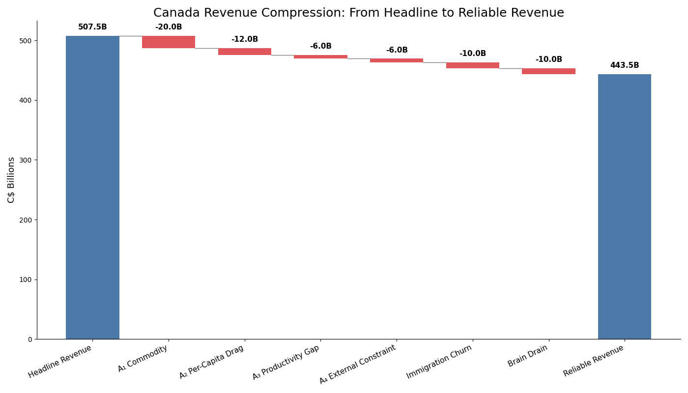
Illustrative revenue compression from headline federal revenue to a more conservative reliable revenue base after adjusting for cyclicality, per-capita drag, productivity weakness, external dependence, immigration churn, and skill drain.
Canada’s resource base is large, but resource abundance does not automatically translate into fiscal strength. The relevant variable is not production volume, but captured value per unit of output.
Oil provides the clearest test case.
Production vs. Pricing
Canada is one of the world’s largest oil producers, but its benchmark, Western Canadian Select (WCS), trades at a persistent discount to West Texas Intermediate (WTI):
- WCS discount to WTI: $12–$20 per barrel
This is direct empirical evidence that production ≠ captured value
Mechanism 1: Infrastructure Constraint
- limited access to non-U.S. markets
- reduced arbitrage opportunity
- dependence on U.S. refining capacity
- crude exported upstream
- value-added stages captured elsewhere
- oil sands are capital-intensive
- higher-cost than conventional crude
- margin capture weaker than headline price implies
Mechanism 4: Fiscal Transmission Limits
- royalties are primarily provincial
- corporate tax is volatile
- boom-bust investment cycles weaken stability
If Canadian oil production is ~4–5 million barrels/day, a $15/bbl discount implies:
Implication
Resource abundance does not guarantee fiscal strength if pricing power, infrastructure access, and value chain participation are constrained.
Figure 2: Canadian Oil’s Realized Price Discount: WTI vs WCS
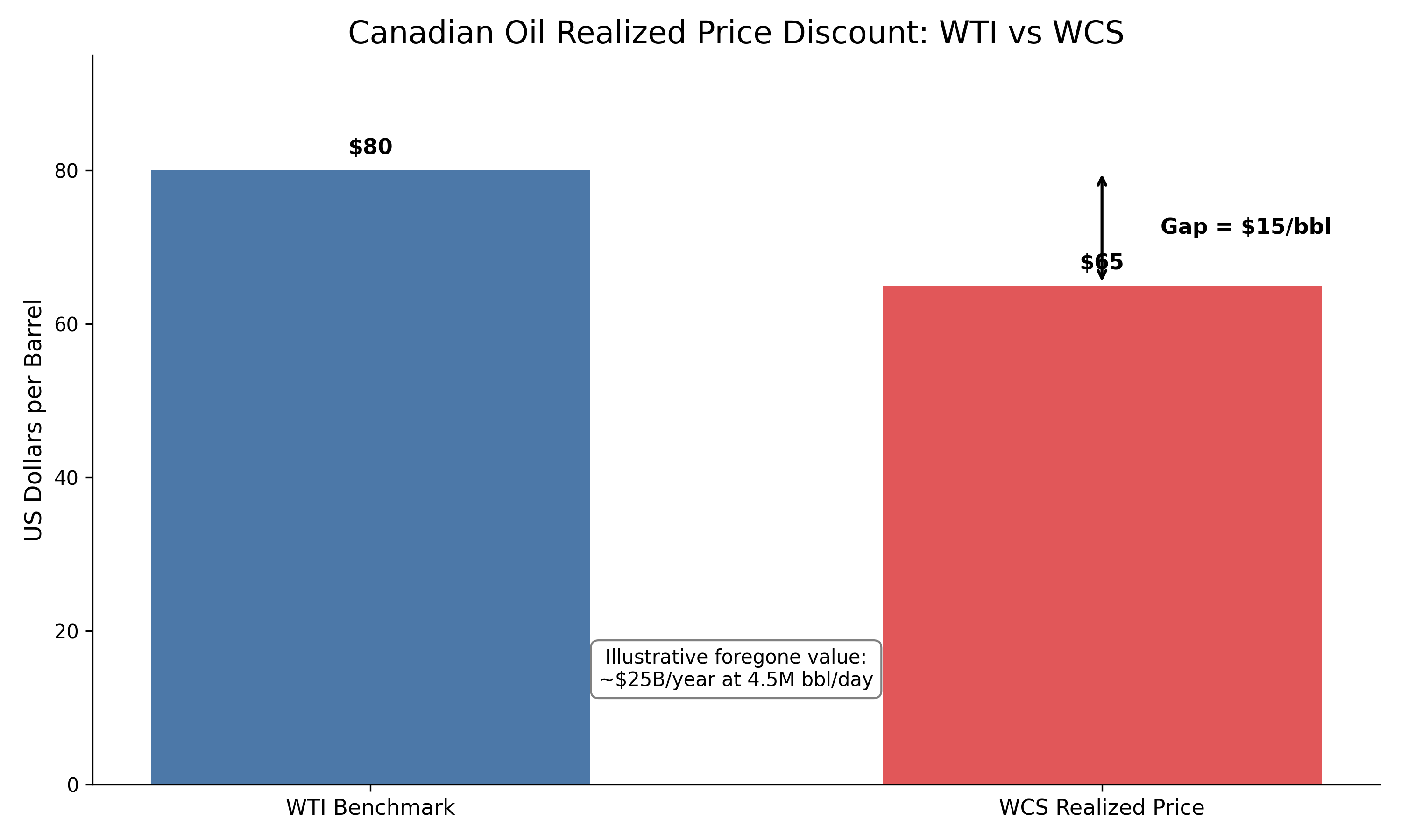
WTI represents the benchmark crude price, while WCS reflects the lower realized price for Canadian heavy crude. The difference is a pricing discount at the point of sale, representing value foregone before it reaches Canadian revenues, profits, or tax receipts.
This is not just oil it is a symptom of a broader retention problem.
From Economic Value Loss to Fiscal Impact
Not all value leakage translates into lost federal revenue.
We define a fiscal transmission factor:
- Effective tax capture rate (τ): ~15–25%
- Reflects corporate tax, royalties, and indirect effects
Example (Oil Discount):
- Gross value gap: ~$25B
- Estimated fiscal impact: ~$4–6B
This conversion ensures that adjustments to \(R_{\text{reliable}}\) reflect tax-relevant losses, not gross production differences.
Bridging Headline to Reliable Revenue (Fiscal vs Economic)
| Adjustment Type | Example | Included in \(R_{\text{reliable}}\)? | Treatment |
|---|---|---|---|
| Direct fiscal | cyclical corporate tax | Yes | Full |
| Tax-transmitted | oil discount (τ applied) | Yes | Scaled |
| Structural economic | pricing power, ownership | No | Context only |
Only tax-transmitted effects are included in \(R_{\text{reliable}}\). Broader economic leakage is used to explain direction, not to directly reduce the denominator.
6.2 The Single‑Customer Constraint
Canada’s external sector is highly concentrated.
- approximately 70–75% of merchandise exports go to the U.S.
- when North America is included, the share rises further
- in energy, autos, and lumber, effective dependence is often higher still
This creates a structural condition:
In a concentrated system:
- one dominant buyer sets the marginal price
- switching costs are asymmetric
- pricing power shifts toward the buyer
Canada–U.S. trade is shaped by:
- geography
- integrated supply chains
- shared infrastructure
- deep regulatory alignment
That makes diversification slower and more expensive than it appears.
Mechanism 3: Policy Sensitivity
Trade concentration makes Canadian policy more sensitive to U.S. preferences:
- softwood lumber disputes
- digital services tax withdrawal
- repeated renegotiations of trade arrangements
Mechanism 4: Integrated Ownership
Beyond goods flows, profits, IP income, and services move across the border.
Mechanism 5: Labor Market Integration
High-skill workers can move or benchmark against the U.S. labor market, weakening domestic pricing autonomy for labor.
Implication
A revenue base concentrated on a single external partner is less autonomous and less resilient than a diversified one.
7. The Population Mask: Why Aggregate Revenue Hides Per‑Capita Constraint
For decades, the structural weaknesses described in Section 5 did not trigger visible fiscal stress. One mechanism absorbed the pressure:
Population growth.
It allowed total revenue to expand even as per‑capita capacity stagnated. Aggregate GDP rose, tax receipts increased, and headline ratios looked stable. But the underlying structure did not improve.
That masking mechanism has now stopped working.
The Arithmetic of the Mask
Revenue is a product of three variables:
Meanwhile:
- Real GDP per capita weakened
- Real wage growth averaged only ~0.53% annually over 43 years
- Housing costs rose 7x faster than wages
Consequence: If population grows at 2% while real productive capacity per person grows at 0–1%, then reliable revenue per capita shrinks in real terms. The aggregate numbers look fine, but the fiscal capacity available per person is declining.
Two Additional Drains
Two measurable outflows compress the denominator further:
- Immigration churn: ~1 in 5 immigrants leaves within 25 years; 36% of foreign‑trained healthcare workers leave within 5 years. Long‑term tax yield is overstated.
- Brain drain: An estimated 800,000–1,000,000 Canadians work in the U.S. (TN visas, permanent moves). This removes high‑earning taxpayers from the domestic base.
Adjusted Reliable Revenue
Including the value capture gap from Section 6, churn, and brain drain:
| Adjustment | Estimated Impact |
|---|---|
| Cyclical & productivity drags | ~$25–40B |
| Value capture gap (oil + services) | ~$35–50B |
| Immigration churn + brain drain | ~$15–25B |
| Total reduction from headline | ~$75–115B |
| Headline revenue | $507.5B |
| Adjusted reliable revenue | ~$390–430B |
At this adjusted base, the true constraint ratio is:
7.1 Regime Shift: When the Population Model Stops Working
For decades, immigration-driven population growth likely supported:
- labor force expansion
- aggregate demand
- tax receipts
- demographic offset
That regime appears to have changed.
Evidence of Regime Breakdown
Despite high immigration, several countervailing forces emerged:
- per-capita GDP stagnation or decline
- weak real wage growth relative to costs
- severe housing burden
- weaker labor market absorption for new entrants
At the same time:
Natural population growth has collapsed, and total population growth has become increasingly dependent on immigration alone.
This creates a structural dependency:
Population growth improves fiscal capacity only if:
Implication
Canada’s population model may not have been inherently flawed, but it appears to have crossed a threshold where additional population no longer translates into increased reliable fiscal capacity.
8. The Mask Comes Off
The previous section argued that immigration’s contribution is now regime-dependent. But the more immediate issue is this:
The population-growth regime has already changed.
- Q4 2025: population fell by 171,296
- Full year 2025: population declined by ~102,000
- 2026 projection: flat growth
This is not a distant forecast. It is a current structural shift.
Figure 3: Canada’s Population Growth Cliff
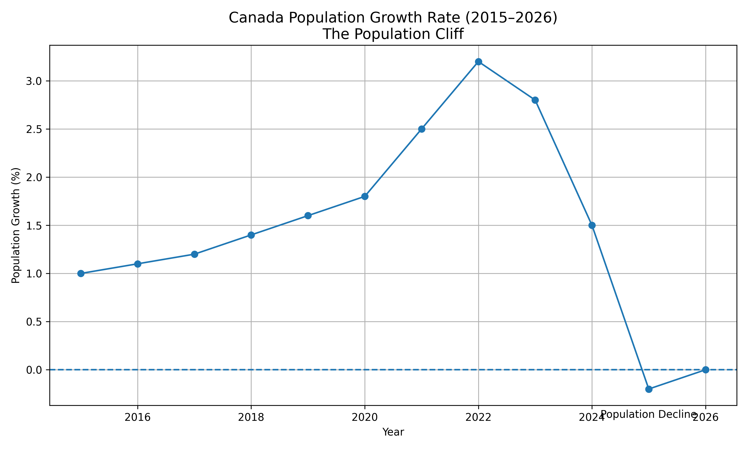
Population growth accelerated through 2023, masking weak per-capita performance. The sharp reversal in 2025–2026 marks the breakdown of the demographic expansion model.
Recalculating ΔS Without Population Growth
Structural revenue growth has three components:
Using a conservative reliable revenue estimate of ~$450B:
| Component | Old Assumption | New Reality |
|---|---|---|
| Real productivity & wage growth | 0.5% | 0.5% |
| Inflation | 2.0% | 2.0% |
| Population growth | 1.5–2.0% | 0% |
| Nominal ΔS | ~$18B | ~$11.25B |
Now compare this to interest repricing pressure:
- federal rate shock: ~$12.2B/year PBO, Debt Sensitivity Analysis, 2025
- provincial refinancing: +$3–5B/year Statistics Canada, Provincial Economic Accounts, Table 36-10-0434-01
- total: ~$15–17B/year
Provincial-federal transmission loop: Provincial fiscal stress transmits to the federal layer through (1) rising equalization and healthcare transfers as provincial revenues weaken under the same demographic and trade constraints, and (2) shared personal/corporate tax bases where provincial rate adjustments or economic contraction directly reduce federal receipts. This feedback loop means provincial refinancing pressure (~$3–5B) is not additive but multiplicative on federal ΔS.
So:
The constraint is not approaching. It is already active.
Figure 4: Crossing of Structural Growth and Interest Pressure (2020–2026)
For most of the past decade, Canada’s fiscal system appeared stable because:
Structural revenue growth (ΔS) exceeded interest pressure (ΔI).
That relationship has now reversed.
With population growth at or near zero, structural revenue growth falls to approximately $10–11B annually**, while interest repricing pressure has risen to **$15–17B. The result is a clear inversion:
This figure plots the rolling 12-month change in structural revenue growth (ΔS) against combined interest pressure (ΔI). For most of the prior decade, ΔS exceeded ΔI, allowing the system to expand despite underlying inefficiencies. In 2025, this relationship reverses: interest growth overtakes structural revenue growth. This crossing marks the transition from apparent stability to active constraint, where new fiscal capacity is no longer sufficient to absorb rising debt service costs.
This crossing is the paper’s central threshold condition. It marks the point at which annual fiscal headroom turns negative.
9. The Threshold
Observed Pattern
| Variable | Trajectory | Driver |
|---|---|---|
| Interest | Rising | Refinancing at higher rates + debt accumulation |
| Headline Revenue | Growing | Legacy population expansion + nominal activity |
| Reliable Revenue | Weaker than it appears | Commodity exposure, productivity gap, external dependence, value leakage |
If revenue quality is overstated, the constraint ratio is understated.
Core Thesis
Canada appears more fiscally stable in aggregate than it is in structural terms because reliable revenue has been overstated and the demographic engine that masked that weakness has stalled.
A Testable Threshold
Following the Ireland framework, define the bind point as:
- Structural revenue growth (ΔS) with flat population: ~$11.25B/year
- Interest repricing pressure (ΔI): ~$15–17B/year
- Revenue shock sensitivity (ΔR) under mild stress: ~$3–5B/year
| Scenario | ΔI + ΔR | ΔS | Status |
|---|---|---|---|
| Baseline (no shock) | ~$15B | ~$11.25B | Constraint active |
| Mild stress (+0.5% rates, -5% corp tax) | ~$18B | ~$11.25B | Severe tightening |
| Severe stress (+1% rates, -10% corp tax) | ~$22B | ~$10B | Critical |
With population growth at zero, the boundary has already been crossed. Interest costs are now growing faster than the system can generate new fiscal capacity.
Operational Definition of the Constraint Threshold
The threshold condition:
- Time basis: rolling 12-month change
- ΔI: change in federal + provincial net interest expense
- ΔS: change in estimated reliable revenue (adjusted)
- ΔR: observed or scenario-based revenue shocks
A crossing is defined as:
Two consecutive periods where (ΔI + ΔR) exceeds ΔS
This ensures the condition reflects a persistent structural shift, not a single-period fluctuation.
Key Refutations & Model Robustness
| Potential Critique | Response |
|---|---|
| “Population growth will resume.” | Possible, but the model only requires one sustained pause for ΔS < ΔI to bind. The system is structurally dependent on uninterrupted expansion. |
| “This is efficient specialization, not leakage.” | Specialization explains trade patterns; persistent WCS discounts and services/IP deficits reflect constrained pricing power, not comparative advantage. |
| “Federal and provincial balance sheets are separate.” | Shared tax bases and equalization mechanics create fiscal transmission. Provincial constraint tightens federal headroom. |
| “The US relationship is strength, not weakness.” | True in expansion, but in concentration, dependency reduces pricing power and policy autonomy. Stability in good times → constraint in stress. |
Figure 5: Canada’s Constraint Phase Diagram
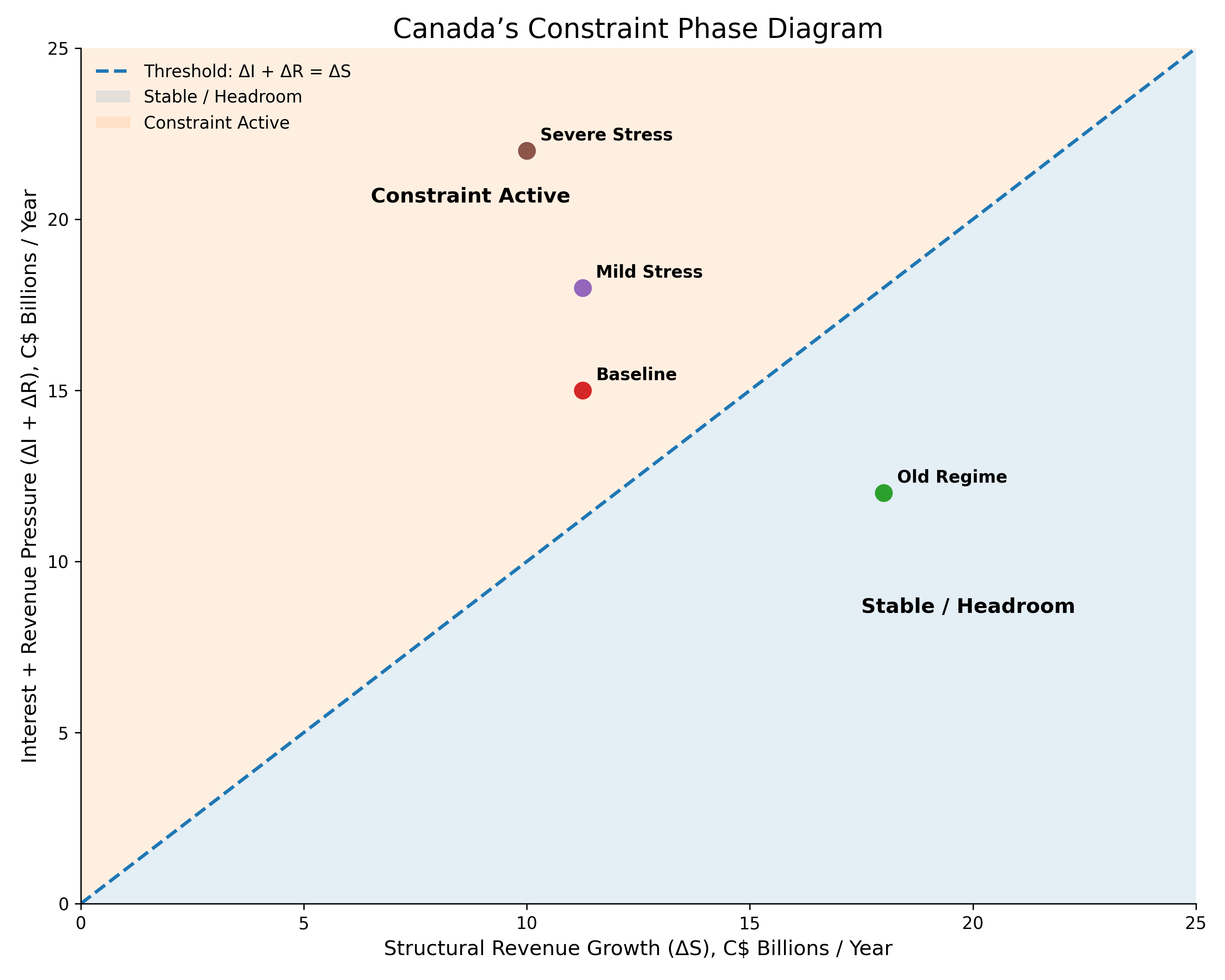
This phase diagram maps Canada’s fiscal position as a function of structural revenue growth (ΔS) and combined annual pressure from interest repricing and revenue shocks (ΔI + ΔR). The diagonal threshold line marks the point where annual fiscal headroom is exhausted. Positions above the line indicate active structural constraint. Canada’s current position, using the paper’s conservative estimates, lies in the constrained region.
With population growth at zero, the boundary has already been crossed. Canada’s annual structural headroom is now approximately -$4B meaning the system is no longer generating enough incremental fiscal capacity to absorb its own rising interest costs.
10. Conclusion
Canada’s challenge is not a future risk. It is a present structural reality.
Three findings emerge from the model:
- Interest costs are rising federal refinancing alone adds ~$15B annually, with provincial and household layers compounding the pressure.
- Reliable revenue is smaller than headline figures suggest because the country does not fully capture and retain the value it produces (see Appendix 4).
- The population-driven expansion has stalled the demographic engine that long supported aggregate growth is no longer doing so.
With zero population growth, the annual increase in structural revenue collapses from ~$18B to ~$11B. Interest pressure already sits at ~$15–17B. The inequality is satisfied before any trade war or recession:
For decades, population growth allowed the system to expand outward. Aggregate revenue rose and fiscal ratios appeared stable, even as underlying per-capita capacity stagnated.
Now, with population growth at zero, the denominator no longer expands fast enough to absorb rising costs. The underlying leakage is exposed, while the cost of past obligations continues to increase. The result is not a sudden crisis, but a system where the margin for error has already been exhausted.
The trade war with the United States is not the cause. It is an accelerant applied to a system already operating at its structural limit.
The constraint did not arrive suddenly. It emerged gradually, and then, with the halt of population growth, all at once.
Canada is not a failing state. But it is now a structurally constrained economy: fixed costs rising, value capture incomplete, and policy flexibility already narrowed.
The question is whether stability can be maintained now that expansion is no longer doing the work.
Where to Go from Here
This is not a prediction of collapse. It is a framework for detecting when stability has already become fragile. The value of the analysis lies in the method:
- decompose the system
- distinguish headline from reliable revenue
- identify denominator distortion
- derive a testable threshold
Forward-looking indicators to monitor:
- Population growth trajectory: If net migration remains flat or negative for >2 consecutive quarters, ΔS remains constrained.
- WCS-WTI spread: A sustained discount >$15/bbl signals continued value leakage.
- Provincial deficit trends: Rising deficits in Ontario, BC, or Alberta increase federal transfer pressure.
- TN visa approvals: Continued high approval rates (>90%) indicate ongoing high-skill outflows.
- Corporate tax concentration: If top-10 firms exceed 60% of federal corporate tax receipts, revenue volatility increases.
Applied to Canada, the result is clear:
The key question is not whether Canada can service its debt. The key question is whether it can do so while retaining the flexibility to absorb shocks, invest in productivity, and support its population without the demographic mask that once hid the strain.
That is the constraint now in view.
Appendix 1: Demographic and Labor Market Dynamics as Fiscal Signals
(Note: This appendix examines how population growth, wage trajectories, mobility patterns, and retention metrics affect the reliability, growth rate, and per-capita capacity of Canada’s revenue base.)
1. The Per-Capita Productivity–Wage Disconnect
Aggregate GDP growth has masked a structural divergence between output, labor compensation, and asset costs. Over the 1981–2024 period:
- Real median hourly wage growth (full-time): +24% total → ~0.53% annualized
- Real inflation-adjusted home price growth: +163.5%
- Result: Housing costs have risen approximately 7x faster than median labor compensation
- Business investment per worker: Lowest among G7 peers while population growth remained elevated
Model Implication: When labor compensation grows near 0.5% annually while fixed costs rise much faster, the personal income tax base expands primarily through population addition, not productivity or real wage growth.
2. Cross-Border Labor Mobility & Human Capital Outflows
Canada’s highest-skill labor cohorts demonstrate measurable exit patterns toward the U.S.:
- TN visa approvals for Canadian professionals remain high
- An estimated 800,000–1,000,000 Canadians reside and work in the U.S.
- Wage and tax differentials remain material in sectors such as engineering, healthcare, technology, and finance
Model Implication: High-skill outflows reduce the domestic tax base per capita and remove human capital required for productivity-led revenue growth.
3. Immigration Retention & Revenue Base Volatility
Canada’s immigration intake expanded significantly, but retention metrics indicate a meaningful churn profile:
- One in five immigrants departs within 25 years
- 36% of internationally educated healthcare workers leave within five years
- Temporary resident outflows rose sharply in 2025
Model Implication: High upfront settlement costs, combined with early attrition of high-education cohorts, reduce the long-term fiscal yield of immigration.
4. Integration with the Constraint Model
| Dynamic | Model Variable Affected | Directional Impact |
|---|---|---|
| Wage stagnation + housing inflation | \(ΔS\) | ↓ Reduces real tax-base expansion |
| High-skill outflows | \(R_reliable\) | ↓ Lowers retention of high-yield cohorts |
| Immigration churn | \(R_reliable\) | ↓ Reduces long-term fiscal yield |
| Low business investment per worker | \(g_R\) | ↓ Suppresses productivity-linked growth |
These dynamics explain why headline revenue growth overstates underlying fiscal capacity.
5. Immigration, Fertility Convergence, and the Limits of Population Replacement
A distinction is needed between population expansion and demographic self-sustainability.
For many years, immigration increased Canada’s population and labor force. But it did not eliminate Canada’s low-fertility problem.
- Permanent resident admissions rose from 272,000 in 2015 to 484,000 in 2024
- 97.3% of population growth in 2025 came from international migration
- Natural increase was only about 19,738 people in 2025
- Total fertility rate fell to 1.25 in 2024
- 42.3% of newborns in 2024 had a foreign-born mother
The implication is not that immigration “does not work.” It is that immigration should be treated as regime-dependent. It can expand population size without fully restoring self-sustaining demographic growth.
| Indicator | 2015 | 2023–2024 / 2025–2026 | What it shows |
|---|---|---|---|
| Permanent resident admissions | 272,000 | 484,000 in 2024 | PR inflows rose sharply |
| Share of population growth from migration | 97.3% in 2025 | Growth overwhelmingly migration-driven | |
| Natural increase | larger historical role | ~19,738 in 2025 | Births minus deaths contribute little |
| Total fertility rate | higher historically | 1.25 in 2024 | Far below replacement |
| Births with foreign-born mother | 42.3% in 2024 | Immigrants still contribute materially | |
| Population growth outlook | pre-2015 avg. 1.1% | flat in 2026; modest medium-term recovery | Higher inflows did not restore durable long-run growth |
Appendix 2: The Value Capture Gap Quantifying the Difference Between Production and Retention
Note: This section estimates the gap between economic value produced within Canada and value retained within the domestic fiscal and income base. These estimates are directional and intended to bound the scale of the effect, not assign precise fiscal loss.
All adjustments to reliable revenue are expressed on a tax-transmitted basis, not gross economic value, ensuring consistency with the federal fiscal denominator.
1. Conceptual Framework
- priced at global benchmarks
- retained within domestic firms
- converted into taxable income
This introduces a gap:
Oil provides the clearest observable estimate of under-capture.
- Production: ~5.13 million barrels/day
- Annualized:
$$ 5.13M \times 365 \approx 1.87 \text{ billion barrels/year} $$ - Average WTI–WCS differential (2024): ~$14–15 USD/bbl
Calculation:
Canada also runs a persistent deficit in:
- services trade
- primary income flows
Estimate:
As % of federal revenue:
| Scenario | Estimated Gap | % Federal Revenue | % GDP |
|---|---|---|---|
| Lower Bound (measured only) | ~$45–50B | ~9–10% | ~1.5–2.0% |
| Moderate | ~$60–80B | ~12–16% | ~2.0–3.0% |
| Upper | ~$90–120B | ~18–24% | ~3.0–4.5% |
7. Interaction with Population Dynamics
At ~40 million population:
- Lower bound (~$48B): **~$1,200 per person**
- Upper bound (~$100B): **~$2,500 per person**
8. Interaction with Interest Growth
9. Key Interpretation
This gap does not represent:
- lost tax revenue
- fully recoverable income
- or simple policy failure
It reflects:
structural limitations in pricing power, ownership, and value chain participation
10. Conclusion
Even under conservative assumptions, the measurable value capture gap is on the order of:
Figure 6. The Value Flow of the Canadian Economy: From Production to Retention
Value leakage occurs at multiple independent stages, meaning even small inefficiencies compound into a large reduction in the effective revenue base.
    flowchart LR
    %% Node definitions with emojis
    A["🏭 Resource Production<br/>Oil, Timber, Minerals"]
    B["💲 Market Pricing"]
    C["🏢 Corporate Ownership"]
    D["👷 Labor Income"]
    E["💰 Taxable Revenue Base"]

    %% Leakage nodes (red)
    L1["📉 Pricing Discount<br/>WCS vs WTI"]
    L2["✈️ Profit Outflows<br/>Foreign Ownership"]
    L3["🧠 Labor Leakage<br/>Brain Drain / US Employment"]
    L4["📜 Services & IP Flows<br/>Cross-Border Deficit"]

    %% Main flow (blue/green tones)
    A --> B --> C --> D --> E

    %% Leakage connections (dashed red)
    B -.-> L1
    C -.-> L2
    D -.-> L3
    C -.-> L4

    %% Styling - Main flow
    style A fill:#2C5F8A,stroke:#1A3F5A,stroke-width:2px,color:#fff,rx:8px
    style B fill:#2C5F8A,stroke:#1A3F5A,stroke-width:2px,color:#fff,rx:8px
    style C fill:#2C5F8A,stroke:#1A3F5A,stroke-width:2px,color:#fff,rx:8px
    style D fill:#2C5F8A,stroke:#1A3F5A,stroke-width:2px,color:#fff,rx:8px
    style E fill:#1E7A5C,stroke:#0E4A3A,stroke-width:3px,color:#fff,rx:8px

    %% Styling - Leakages (red/orange)
    style L1 fill:#C23B22,stroke:#8B2A18,stroke-width:2px,color:#fff,rx:8px
    style L2 fill:#C23B22,stroke:#8B2A18,stroke-width:2px,color:#fff,rx:8px
    style L3 fill:#C23B22,stroke:#8B2A18,stroke-width:2px,color:#fff,rx:8px
    style L4 fill:#C23B22,stroke:#8B2A18,stroke-width:2px,color:#fff,rx:8px

    %% Link styles
    linkStyle default stroke:#5A9EC2,stroke-width:2px
    linkStyle 4 stroke:#C23B22,stroke-width:2px,stroke-dasharray: 5 5
    linkStyle 5 stroke:#C23B22,stroke-width:2px,stroke-dasharray: 5 5
    linkStyle 6 stroke:#C23B22,stroke-width:2px,stroke-dasharray: 5 5
    linkStyle 7 stroke:#C23B22,stroke-width:2px,stroke-dasharray: 5 5
This diagram illustrates how economic value generated within Canada flows through multiple stages before becoming government revenue. At each stage pricing, ownership, labor, and services a portion of that value is not retained within the domestic economy. These leakages reduce the effective tax base and help explain why reliable revenue is structurally lower than headline figures suggest.
Synthesis: Evidence of Systematic Under-Capture
The conclusion that Canada does not fully capture the value it produces is not based on a single assumption. It emerges from three independent, observable mechanisms:
-
Commodity pricing differentials → Canadian oil is consistently sold below global benchmark prices → Direct evidence of foregone value at the point of sale
-
Services and income flow deficits → Profits, intellectual property income, and service revenues accrue outside Canada → Value is produced domestically but realized externally
-
Labor and capital mobility → High-skill workers and capital migrate toward higher-return environments → The highest-value segments of production are not retained within the domestic tax base
These effects operate across different layers of the economy pricing, ownership, and labor but produce the same outcome:
Reliable revenue is structurally lower than headline figures imply because the economy does not fully capture and retain the value it generates. This is the paper’s central empirical claim.
Canada’s constraint is not primarily driven by insufficient production, but by systematic under-capture of the value it produces across pricing, ownership, and labor channels.
Appendix 3: Triple Compression Forward Stress Framework
(Note: A stress framework evaluating how Canada’s fiscal constraint behaves under simultaneous pressure from rising interest costs, weakening population growth, and persistent value-capture leakage.)
1. Framework Overview
Combining them:
(1) Interest Pressure
| Variable | Value |
|---|---|
| Headline federal revenue | C$507.5B |
| Federal net interest | C$54B |
| Conservative reliable revenue | ~C$450B |
| Lower-bound value gap | ~C$45–50B |
| Fertility rate (2024) | 1.25 |
| Population outlook | Flat (near-term baseline) |
4. Scenario Design
| Scenario | Fertility | Population Trend | Interest Shock | Value Gap |
|---|---|---|---|---|
| Base | 1.25 | Flat / modest growth | Current | C$50B |
| Stress | 1.10 | Flat to mildly negative | +10% | C$75B |
| Severe | 1.00 | Declining (~1%) | +20% | C$100B |
5. Calculation Method
Step 1 Adjust Revenue for Value Leakage:
| Scenario | Adjustment |
|---|---|
| Base | 0% |
| Stress | -2% |
| Severe | -5% |
Step 3 Adjust Interest:
| Scenario | Interest |
|---|---|
| Base | C$54.0B |
| Stress | C$59.4B |
| Severe | C$64.8B |
6. Triple Compression Results
| Scenario | Headline Revenue | Value Gap | Demographic Drag | Effective Revenue | Interest | Constraint Ratio |
|---|---|---|---|---|---|---|
| Base | 507.5 | 50 | 0% | 457.5 | 54.0 | 11.8% |
| Stress | 507.5 | 75 | -2% | 424.2 | 59.4 | 14.0% |
| Severe | 507.5 | 100 | -5% | 387.1 | 64.8 | 16.7% |
7. Interpretation
The system compresses when:
- interest rises
- population growth no longer expands the tax base
- economic value is not fully retained
This produces:
| Value Gap | Per-Capita Equivalent |
|---|---|
| C$50B | ~$1,250 |
| C$75B | ~$1,875 |
| C$100B | ~$2,500 |
9. Model Implication
The condition
- $\Delta S$ weakens due to demographic slowdown
- $\Delta R$ is hit by value leakage
- $\Delta I$ rises due to refinancing
10. Conclusion
Canada’s fiscal constraint is shaped not by one variable, but by the interaction of rising interest costs, weakening demographic support, and incomplete value capture.
Even under moderate assumptions, these forces compress fiscal flexibility over time.
Appendix 4: Quantifying the Value Capture Gap A Lower‑Bound Observable Estimate
This appendix demonstrates, using publicly available data, that a significant portion of economic value produced in Canada does not translate into domestically controlled, reliable revenue. The calculation is a lower bound it includes only components that can be directly observed or conservatively estimated. Broader structural factors (cyclicality, productivity drag, immigration churn, brain drain) would increase the gap further.
| Component | Annual Estimate (CAD) | Source / Basis | Calculation |
|---|---|---|---|
| 1. Oil pricing discount (WCS vs. WTI) | ~$25 billion | WCS‑WTI spread: $12–20/barrel (Fitch, industry reports). Production: ~4.5 million barrels/day (Canada Energy Regulator). | 4.5M bbl/day × 365 days × $15 midpoint = ~$24.6B |
| 2. Services trade deficit | ~$3.6 billion | Statistics Canada, Q1 2025 quarterly deficit ~$0.9B | $0.9B × 4 quarters = $3.6B |
| 3. Primary income deficit (profits, dividends, IP royalties) | ~$2.0 billion | Statistics Canada, Q1 2025 quarterly deficit ~$0.5B | $0.5B × 4 quarters = $2.0B |
| 4. Foreign profit outflows (conservative) | ~$5 billion | Foreign‑controlled firms hold ~14.4% of Canadian corporate assets (Statistics Canada, Corporations Returns Act 2023). A portion of their profits is repatriated. | Conservative estimate; actual could be higher |
| Lower‑bound observable value capture gap | ~$36 billion | Sum of above | ~7% of federal revenue ($507.5B) |
Notes:
- This gap represents foregone economic value before any taxes are applied. It directly reduces the pool of income available for corporate taxes, personal income taxes (wages, bonuses), and consumption taxes.
- The oil discount alone accounts for ~70% of the observable gap. It is not a political claim it is a daily market price differential published by commodity exchanges.
- Broader structural factors (cyclical commodity dependence, productivity gap, per‑capita drag, immigration churn, brain drain) would increase the total gap to an estimated 15–20% of headline revenue (~$75–100B). See Section 6 and Appendix 1 for discussion of those factors.
Appendix 5: AI‑Assisted Reasoning Process (Summary)
Note: This appendix documents the iterative, multi‑model process that revealed Canada’s fiscal constraint is already active—placing it in a structurally worse position than Ireland or the United States.
The Process in Five Phases
Phase 1: Reframing the Problem
- Started with a contradiction: Canada appears highly dependent on the US, yet trade friction persists
- Rejected simplistic “vassal state” narratives; focused on structural outcomes over conspiracy
- Discovered Canada’s constraint differs from US (interest velocity) and Ireland (accounting gap)
Phase 2: Uncovering Hidden Variables
- Transformed social indicators (wage stagnation, housing costs) into core model inputs
- Reframed immigration as regime-dependent: expansionary when absorptive capacity is strong, dilutive when infrastructure/productivity lag
- Identified measurable value leakage: WCS-WTI oil discount (~$25-38B annually) and single-customer concentration (70-75% exports to US)
Phase 3: The Critical Discontinuity
- Key breakthrough: Population growth fell in Q4 2025 and projected flat in 2026
- This collapsed structural revenue growth (ΔS) from ~$18B to ~$11.25B annually
- Interest pressure (ΔI) remained at $15-17B, satisfying the constraint inequality
ΔI + ΔR ≥ ΔSbefore any shock - The masking mechanism had already stopped working
Phase 4: Integration & Quantification
- Decomposed debt into three layers (federal, provincial, household) revealing systemic transmission
- Applied churn/brain drain adjustments (~$8-12B revenue drag)
- Calculated Canada’s fiscal headroom at ~-$4B (vs Ireland’s +€4.2B)
Phase 5: Narrative Synthesis
- Restructured analysis as detective story: apparent stability → hidden leakages → regime shift → active constraint
- Added adversarial validation throughout
- Final conclusion: “Canada is constrained not because it produces too little, but because it captures too little—and the mechanism that hid that gap has stopped working.”
Why Canada Was Harder
| Dimension | Ireland | United States | Canada |
|---|---|---|---|
| Hidden distortion | One accounting gap (GNI*) | Interest velocity | Regime shift + multiple leakages |
| Signal clarity | Single number (~43%) | Clear differential | Weak signals cohering only when population stalled |
| AI disagreement | Low | Low | High (three competing hypotheses) |
The Canadian case required synthesising three independent perspectives (value capture, demographics, trade concentration) and recognising that population growth was a regime parameter, not a continuous variable.
Reproducibility Checklist
To replicate this analysis for any complex system:
- Start with a real-world inconsistency
- Decompose into measurable layers
- Stress-test assumptions adversarially
- Use multiple AI models to identify divergent hypotheses
- Anchor all claims in official data
- Derive a testable threshold condition
- Write as detective story, not report
Result: A framework revealing that Canada’s constraint is already active a finding that emerged only when population growth was treated as a discontinuous regime shift rather than a continuous variable.
Appendix 6: Adversarial Checks and Potential Refutations
1. “Canada Specializes Efficiently This Isn’t Leakage”
Criticism:
Canada exports raw resources because it is economically optimal.
Response:
-
Specialization explains some structure
-
But persistent price discounts (WCS vs WTI) are not specialization
-
They reflect:
- constrained market access
- buyer concentration
- limited pricing power
Conclusion: This is not neutral specialization it is constrained value capture.
2. “Population Growth Will Resume”
Criticism:
The 2025–2026 slowdown is temporary.
Response:
- Possible and explicitly acknowledged in the model
- But the key point:
The system only works if population growth is continuous
If growth pauses:
- ΔS collapses immediately
- ΔI continues rising
Conclusion: The system is structurally dependent on uninterrupted expansion.
3. “Federal vs Provincial Separation Protects Canada”
Criticism:
Federal debt is manageable; provinces are separate.
Response:
-
Provinces control:
- healthcare
- infrastructure
-
Already running deficits (e.g., BC, Ontario)
In stress:
Federal transfers rise → Federal denominator absorbs provincial stress Conclusion: The separation is accounting, not economic reality.
4. “The US Relationship Is Strength, Not Weakness”
Criticism:
Integration with the US provides stability.
Response:
- True in expansion
- But in concentration:
Dependency reduces pricing power and policy autonomy
Conclusion: Stability in good times → constraint in stress.
Appendix 7: Formal Derivation of the Constraint Inequality
This appendix derives the central condition \(\Delta I + \Delta R \geq \Delta S\)
from the government’s intertemporal budget constraint. The derivation shows that the inequality is not an arbitrary heuristic but a stability condition for a sovereign borrower with limited control over its effective revenue base.
1. Starting Point: The Government Budget Constraint
Let:
- \(G_t\) = primary government spending (excludes interest)
- \(I_t\) = interest payments on outstanding debt
- \(R_t\) = total government revenue
- \(D_t\) = gross debt at end of period \(t\)
- \(r_t\) = effective nominal interest rate on debt
In any period:
2. Introduce the “Reliable Revenue” Concept
Define reliable revenue \(S_t\) as the portion of \(R_t\) that is:
- Structurally persistent
- Domestically generated
- Not subject to cyclical or external concentration risk
Then:
3. Interest Dynamics
Debt evolves as:
4. Stability Condition
A fiscally sustainable system requires that the debt‑to‑revenue ratio does not explode. A sufficient (not necessary) condition is:
Substitute \(\Delta D_t = G_t + I_t - R_t\):
Simplify: set \(G_t = \bar{G}\) (constant for the margin analysis). Then:
The inequality is derived, not assumed. It states:
A sovereign borrower that cannot reduce primary spending further will face an active fiscal constraint when the annual increase in interest costs, plus any negative revenue shock, exceeds the annual increase in its reliable revenue base.
The paper applies this to Canada by measuring \(\Delta I\) from refinancing pressure, \(\Delta R\) from trade or cyclical shocks, and \(\Delta S\) from population, productivity, and inflation.
6. Why Linear Approximation for \(\Delta S\) Is Conservative
In the main paper, \(\Delta S = S \times (g_{pop} + g_{prod} + g_{inf})\). The exact compounding would be:
Appendix 8: Policy Implications Restoring Fiscal Headroom
This appendix translates the paper’s diagnosis into actionable policy levers. Each lever targets a specific leakage or constraint mechanism identified in the main analysis.
1. Closing the Value Capture Gap
The paper estimates an observable value capture gap of ~$36–50B annually (oil discount + services/income deficits + profit outflows). Not all of this is recoverable, but a portion is.
| Mechanism | Policy Lever | Estimated Annual Fiscal Benefit |
|---|---|---|
| Oil pricing discount (WCS vs WTI) | Expand tidewater access (e.g., LNG, pipeline diversification) to reduce single‑customer pricing power. | ~$4–6B (fiscal share of $15‑20B price improvement) |
| Services & IP deficit | Targeted R&D tax incentives to retain intellectual property in Canada; review transfer pricing rules. | ~$1–2B |
| Foreign profit outflows | Reduce barriers to Canadian ownership in resource sectors; consider progressive repatriation incentives. | ~$2–3B |
| Total potential recovery | ~$7–11B / year |
This would reduce the constraint ratio from ~13.5% to ~11–12%, moving the system back toward the threshold.
2. Restoring Demographic Headroom Without Population Growth
The paper shows that zero population growth collapses \(\Delta S\) from ~$18B to ~$11B. If population cannot be forced to grow, productivity must replace it.
| Target | Current | Required | Policy Pathway |
|---|---|---|---|
| Real GDP per capita growth | ~0.5% | ~1.5% | Business investment tax credits; reduce interprovincial trade barriers; streamline major project approvals |
| Labor force participation (prime age) | ~85% | ~88% | National childcare and eldercare infrastructure (already underway, needs acceleration) |
| Immigration retention | 1 in 5 leave within 25 years | Reduce to 1 in 10 | Settlement supports, credential recognition, housing‑linked immigration targets |
If productivity growth doubles to 1.0% (not heroic), \(\Delta S\) rises by ~$4.5B/year — enough to close half the current deficit.
3. Reducing Interest Sensitivity, Lowering \(\Delta I\)
The paper treats \(\Delta I\) as exogenous to policy in the short run, but two levers exist:
- Extend debt maturity: Canada’s average maturity (~6–7 years) is shorter than the UK (~15 years). Lengthening to 10+ years reduces annual repricing pressure.
- Provincial coordination: Create a federal–provincial debt issuance council to avoid crowding out and manage refinancing schedules jointly.
Estimated impact: reduces \(\Delta I\) by ~$1–2B/year under a +1% rate shock.
4. Building a Buffer Against \(\Delta R\) Shocks
The paper notes that a US trade war or commodity price drop adds \(\Delta R\) (negative revenue shock). To absorb such shocks without breaking the constraint:
| Shock Type | Recommended Buffer | Cost |
|---|---|---|
| US tariff escalation (5% of GDP) | Stabilization fund financed by resource royalties | Build to $20B over 5 years |
| Corporate tax volatility | Cap revenue forecasting at 5‑year rolling average; budget conservatively | Zero fiscal cost (prudential) |
5. Monitoring the Threshold in Real Time
The paper’s forward indicators are good. Add a traffic light system for policy makers:
| Indicator | Green (headroom) | Yellow (watch) | Red (constraint active) |
|---|---|---|---|
| \(\Delta I + \Delta R - \Delta S\) | < -$5B | -$5B to $0B | > $0B |
| Population growth (q/q) | >0.5% | 0–0.5% | Negative |
| WCS‑WTI spread | <$10 | $10–$15 | >$15 |
| Provincial deficit trend | Falling | Flat | Rising 2+ quarters |
6. What the Paper Does Not Recommend
- Austerity for its own sake (the constraint is structural, not cyclical)
- Breaking trade ties with the US (concentration is a risk, but diversification takes decades)
- Blaming immigration (the problem is absorptive capacity, not inflow levels)
7. Estimated Total Improvement Path
| Intervention | Annual Headroom Improvement |
|---|---|
| Value capture recovery (moderate) | +$5B |
| Productivity growth (+0.5%) | +$2.25B |
| Extended debt maturity | +$1.5B |
| Provincial coordination | +$0.5B |
| Total | +$9.25B |
The current headroom is approximately -$4B**. A combined policy package of the type outlined above would bring headroom to **+$5B, moving Canada from “constraint active” to “safe buffer.”
8. A Border Work City: A Shenzhen‑Style Economic Zone for Demographic and Value‑Capture Relief
One proposal that emerges directly from the paper’s logic is a purpose‑built, work‑focused city near a major Alberta–US border crossing (e.g., Coutts or a new greenfield site). The design would break from traditional immigration and housing models:
- Unrestricted US access US citizens can live, work, and invest in the city without additional visas.
- Job‑linked automatic visa status Any person (from any country) who secures a legitimate job offer in the city receives an automatic work visa and residency permit for the zone. No points system, no family sponsorship backlog.
- Business‑first land use The city is not a suburb. It is high‑density rental housing, industrial parks, logistics hubs, and cross‑border service centres. Land is publicly owned and leased, not sold, to keep rents low.
- Fresh‑start mandate The city explicitly markets itself to people who want to restart their lives: immigrants, displaced workers, young families priced out of Toronto/Vancouver, even Americans seeking a different economic environment. To attract employers, the zone offers a 10‑year corporate tax holiday on new value‑added activities (manufacturing, logistics, R&D) and streamlined regulatory approval for export‑oriented production.
Underlying logic: Canada’s demographic mask fell when population growth stalled. Adding people to overheated, low‑productivity‑growth cities no longer expands ΔS efficiently. A new city resets the marginal cost of population growth and captures value at the border instead of leaking it to the US.
How It Addresses the Paper’s Constraint
Recall the active constraint:
| Paper’s problem | How the border work city helps |
|---|---|
| Population growth stalled (ΔS collapsed) | Adds net new residents without competing for housing in existing cities. Even 200,000–300,000 people in the zone would restore positive population growth, raising ΔS by ~$2–3B/year once mature. |
| Value capture gap (oil discount, services deficit) | Shifts activity from raw resource exports to value‑added production (assembly, processing, cross‑border logistics) inside the zone, where corporate and personal taxes are captured by Canada. |
| Immigration churn and brain drain | Gives skilled and semi‑skilled workers a low‑cost, low‑friction entry point. The job‑linked visa reduces the incentive to move to the US immediately, improving retention. |
| Housing as a tax drag | Cheap rental housing (public land, high density) means more disposable income → stronger consumption tax base, less household debt stress. |
| US trade concentration risk | Paradoxically, the city uses US proximity to capture activity that currently happens on the US side of the border. It does not reduce concentration, but it changes the terms from passive dependence to active capture. |
Estimated Fiscal Impact (Order‑of‑Magnitude)
| Timeframe | Population added | ΔS contribution | Value‑capture uplift | Net headroom improvement |
|---|---|---|---|---|
| 0–5 years (construction) | ~50,000 | ~$0.5B (net, after infrastructure debt service) | ~$0.5B | ~$1B (mostly reinvested) |
| 6–10 years (early operation) | ~200,000 | ~$2B | ~$1.5B | ~$3.5B |
| 10–20 years (mature) | ~500,000 | ~$4B | ~$3B | ~$7B |
Note: Upfront infrastructure debt increases ΔI temporarily. Phased construction over 10–15 years, funded by a dedicated development bond, would keep annual ΔI manageable.
Risks and Mitigations
| Risk | Mitigation |
|---|---|
| Upfront fiscal cost (tens of billions) | Phase construction; use land lease revenues to service debt; federal‑provincial cost split with Alberta. |
| Crowd‑out of other regions | Explicitly cap zone population at 1% of national total for first decade, then review. |
| US unilateral action (e.g., closing border crossing) | Design zone with redundant transport links (rail, air, secondary crossings). Negotiate a bilateral CUSMA annex. |
| Indigenous land rights | Mandate co‑ownership or revenue sharing with local First Nations (Treaty 7 or 8). No construction without consent and benefit agreement. |
| Becoming a low‑wage enclave | Apply federal labour standards and union access; zone does not exempt employers from Canadian law. |
| Housing still inflates | Public land leasing, not selling. Rent controls indexed to zone wages. |
Why This Is Not a Standard Policy Recommendation
This proposal is radical by Canadian standards. It borrows from Shenzhen (China), Songdo (South Korea), and special economic zones in the UAE. It explicitly rejects the incrementalism of “build more housing in existing cities” and “tweak immigration points.”
But the paper’s own model shows that incrementalism no longer works. The demographic regime has shifted. Value leakage is structural. A border work city is not a short‑term fix — it is a 20‑year structural investment that directly addresses the collapse of ΔS and the value capture gap.
Bottom line: If the paper’s diagnosis is correct (Canada is structurally constrained, not cyclically), then the policy response cannot be marginal. A purpose‑built work city on the US border is one of the few proposals that matches the scale of the problem.
Appendix 9: Comparative Benchmarks How Canada Differs from Peers
| Country | Value Capture Indicator | Demographic Trend | ΔI vs ΔS Status |
|---|---|---|---|
| Norway | Oil sold at Brent parity (no discount); sovereign wealth fund captures windfalls | Fertility 1.5, positive net migration | Positive headroom |
| Australia | Resources sold at global prices; diversified export partners (China, Japan, Korea) | Fertility 1.6, strong immigration retention | Near threshold but not crossed |
| Canada | Persistent WCS discount (12‑20% below WTI); 75% exports to US | Fertility 1.25, population fell in 2025 | Constraint active |
The gap is not inevitable. Norway and Australia show that value capture and demographic resilience can be improved. Canada’s current position is an outcome of policy choices and infrastructure constraints, not geography or destiny.
📚 Suggested Citation
Ernan Hughes. (2026). Canada: When Interest Meets Reliable Revenue.
Available at: https://programmer.ie/post/canada/
Version: 1.0
Date: April 2026
⚖️ License
This document is intended as a working paper and may be updated as new data or assumptions evolve.
This work is licensed under the Creative Commons Attribution-NonCommercial 4.0 International License (CC BY-NC 4.0).
You are free to:
- Share — copy and redistribute the material in any medium or format
- Adapt — remix, transform, and build upon the material
Under the following terms:
- Attribution — You must give appropriate credit
- NonCommercial — You may not use the material for commercial purposes
Full license: https://creativecommons.org/licenses/by-nc/4.0/
