Cellular Automata From First Principles 06: Patterns as Data — Oscillators, Spaceships and Gliders

Once we can run Conway’s Game of Life, the next step is not to add more graphics.

It is to make the patterns themselves inspectable.

A blinker is not interesting because somebody named it.

It is interesting because it returns to the same state after two generations.

A glider is not interesting because it has a familiar shape.

It is interesting because the same local configuration reappears after several generations at a translated position.

Those are properties we can test.

Store patterns explicitly

import numpy as np

PATTERNS = {
    "block": np.array([
        [1, 1],
        [1, 1],
    ], dtype=np.uint8),

    "blinker": np.array([
        [1, 1, 1],
    ], dtype=np.uint8),

    "glider": np.array([
        [0, 1, 0],
        [0, 0, 1],
        [1, 1, 1],
    ], dtype=np.uint8),
}

The canonical figure for this chapter is generated from exactly those three patterns:

python scripts/figures/cellular-automata/part01_foundations.py 06

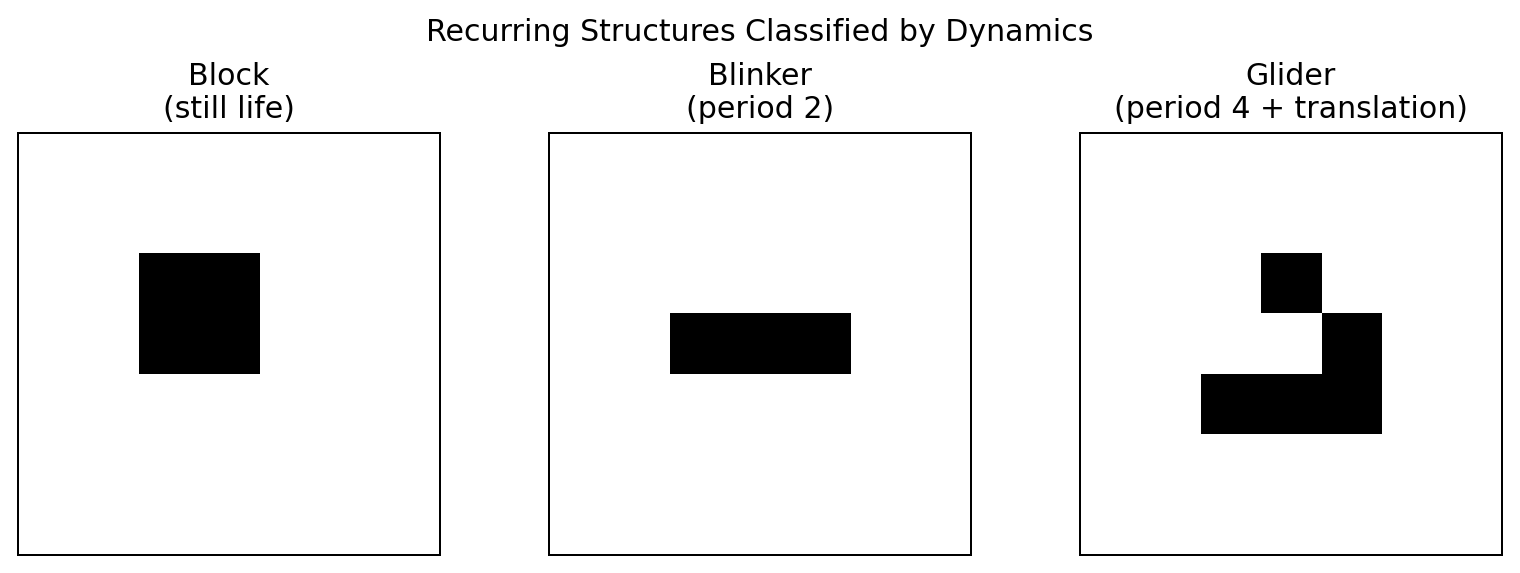
Now create a helper that places a pattern into a larger world:

def place(grid, pattern, row, col):
    h, w = pattern.shape
    grid[row:row+h, col:col+w] = pattern

This tiny abstraction changes our workflow.

We can now construct experiments from named initial conditions instead of repeatedly editing coordinates.

Crop a pattern to its live bounding box

To compare patterns independently of empty space, crop away dead borders:

def crop_live(grid):
    rows, cols = np.where(grid == 1)

    if len(rows) == 0:
        return np.zeros((0, 0), dtype=np.uint8)

    return grid[
        rows.min():rows.max() + 1,
        cols.min():cols.max() + 1,
    ]

That lets us compare the intrinsic pattern rather than its absolute position.

There is an important limitation: cropping removes location but not rotation or reflection. That is fine for our first classifier, as long as we know exactly what invariance we have introduced.

Detect a still life

A still life is simply a fixed point:

F(state) = state

Test it directly:

def is_still_life(grid):
    return np.array_equal(grid, life_step(grid))

A block should pass.

This is the first important shift from visual inspection to executable classification.

Detect an oscillator period

def oscillator_period(grid, max_period=20):
    initial = grid.copy()
    state = grid.copy()

    for period in range(1, max_period + 1):
        state = life_step(state)
        if np.array_equal(state, initial):
            return period

    return None

For a blinker placed in a sufficiently large world:

period = oscillator_period(grid)
print(period)

should produce:

2

The phrase “sufficiently large” matters because our life_step() currently uses periodic boundaries. If a pattern reaches an edge, wraparound becomes part of the experiment.

The definition has become code.

Detect translation

A spaceship repeats its shape after moving.

One simple approach is to crop the live cells:

def normalized_shape(grid):
    return crop_live(grid)

Then track the top-left position of the live bounding box:

def live_origin(grid):
    rows, cols = np.where(grid == 1)
    if len(rows) == 0:
        return None
    return int(rows.min()), int(cols.min())

Now evolve until the shape repeats:

def find_translation_cycle(grid, max_steps=20):
    initial_shape = normalized_shape(grid)
    initial_origin = live_origin(grid)
    state = grid.copy()

    for step_number in range(1, max_steps + 1):
        state = life_step(state)

        if np.array_equal(normalized_shape(state), initial_shape):
            origin = live_origin(state)
            displacement = (
                origin[0] - initial_origin[0],
                origin[1] - initial_origin[1],
            )
            return step_number, displacement

    return None

For our glider orientation, this reports the key dynamical fact:

period = 4
non-zero displacement

The exact displacement sign depends on the orientation and coordinate convention, so the reusable classifier should report it rather than hard-code a verbal direction.

Why this matters

The grid contains only bits.

Our analysis layer introduces concepts such as:

object identity
period
velocity
persistence
collision

Those concepts are not stored inside individual cells.

They are descriptions of patterns across space and time.

This is an important general technique:

When a low-level system develops recurring structure, build measurements at the level where the recurring structure exists.

Do not force every useful concept into the primitive representation.

Collision experiments

Once patterns are data, we can generate experiments systematically.

def make_world(height=80, width=120):
    return np.zeros((height, width), dtype=np.uint8)

world = make_world()
place(world, PATTERNS["glider"], 10, 10)
place(world, np.fliplr(PATTERNS["glider"]), 10, 80)

Now simulate and record:

history = simulate_life(world, 200)

We can ask:

• do the patterns survive?
• how many live cells remain?
• does the final state become periodic?
• are new moving structures emitted?

A collision therefore becomes a reproducible experiment rather than an animation we happened to watch once.

Pattern fingerprints

We can create a basic fingerprint:

def fingerprint(grid):
    cropped = crop_live(grid)
    return (
        cropped.shape,
        int(cropped.sum()),
        cropped.tobytes(),
    )

For rotation- or reflection-invariant matching, generate transformed versions and choose a canonical representation.

For translation-invariant temporal matching, compare cropped shapes while separately retaining origin and time.

Those distinctions matter because “same pattern” is not one universal equivalence relation. We have to define what changes we want the identity test to ignore.

That gives us the beginning of a pattern database.

Later, similar ideas will help us catalogue emergent structures in less familiar automata where nobody has already supplied names.

From named objects back to rules

It is tempting to look at Life and think the interesting things are gliders, blinkers and spaceships.

But remember the causal direction:

B3/S23
  |
local updates
  |
recurring structures
  |
our higher-level names

The objects are consequences of the rule.

That means changing the rule can create an entirely different ecology of structures.

In the next chapter we will do exactly that: keep the same grid and neighborhood, but move beyond Conway’s Life into other Life-like cellular automata and multi-state rules.