Cellular Automata From First Principles 07: Beyond Conway — Life-like and Multi-State Rules

Conway’s Game of Life is famous enough that it can accidentally become the definition of cellular automata.

It is not.

Life is one point in a much larger design space.

Keep the same two-dimensional grid and the same eight-cell Moore neighborhood, then change only the birth and survival counts.

You immediately get a family of Life-like cellular automata.

Then add more than two cell states and the design space expands again.

This chapter turns the rule itself into data so we can explore that space systematically.

Generalize B3/S23

Life is:

B3/S23

Represent the birth and survival counts as sets:

LIFE_BIRTH = {3}
LIFE_SURVIVE = {2, 3}

Then write one general transition function:

def life_like_step(grid, birth, survive):
    n = neighbor_count(grid)

    born = (grid == 0) & np.isin(n, list(birth))
    stays_alive = (grid == 1) & np.isin(n, list(survive))

    return (born | stays_alive).astype(np.uint8)

Conway’s rule becomes:

grid = life_like_step(grid, birth={3}, survive={2, 3})

The engine no longer knows anything about Conway.

It knows only how to apply a totalistic birth/survival rule.

HighLife

HighLife uses:

B36/S23

The only difference from Conway’s Life is that dead cells are also born when they have six live neighbors.

next_grid = life_like_step(
    grid,
    birth={3, 6},
    survive={2, 3},
)

One extra birth condition changes the available long-term structures. HighLife is particularly well known for supporting a small self-replicating pattern.

That is exactly the kind of experiment cellular automata are good at:

small rule change
      |
      v
large behavioral change

Seeds

Seeds uses:

B2/S

Cells never survive.

A dead cell is born if it has exactly two live neighbors.

next_grid = life_like_step(
    grid,
    birth={2},
    survive=set(),
)

This creates a very different world because every live cell is guaranteed to disappear at the next generation.

Persistence must therefore exist as propagation rather than individual survival.

That distinction is worth noticing.

A stable high-level process does not require stable low-level components.

Compare rules under the same initial condition

rng = np.random.default_rng(42)

grid = (rng.random((120, 160)) < 0.25).astype(np.uint8)

Run the same initial grid under several rules:

rules = {
    "Life": ({3}, {2, 3}),
    "HighLife": ({3, 6}, {2, 3}),
    "Seeds": ({2}, set()),
}

The canonical figure holds the initial condition, grid, neighborhood, boundaries and number of generations constant. Only the rule changes:

python scripts/figures/cellular-automata/part01_foundations.py 07

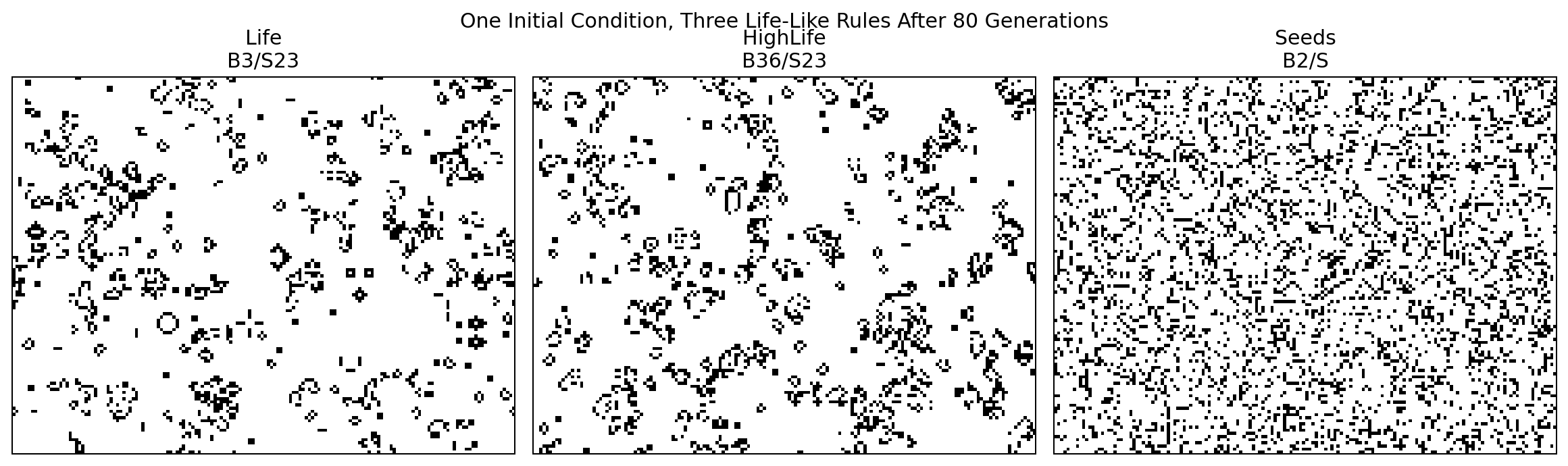
That controlled comparison is much more informative than looking at three unrelated screenshots.

Record population curves

def population_curve(initial, birth, survive, steps=200):
    state = initial.copy()
    values = []

    for _ in range(steps):
        values.append(int(state.sum()))
        state = life_like_step(state, birth, survive)

    return values

Now rule comparison becomes an experiment rather than a visual impression.

Population is only one observable. Two rules can have similar population curves while producing very different spatial organization, which is why later chapters add richer measurements.

Add a third state

Binary states are not required.

Consider a cell with three states:

0 = ready
1 = firing
2 = refractory

A simple excitable automaton can update like this:

def excitable_step(grid):
    firing = (grid == 1).astype(np.uint8)
    firing_neighbors = neighbor_count(firing)

    next_grid = np.zeros_like(grid)

    # firing -> refractory
    next_grid[grid == 1] = 2

    # refractory -> ready
    next_grid[grid == 2] = 0

    # ready -> firing if exactly two neighbors fire
    activate = (grid == 0) & (firing_neighbors == 2)
    next_grid[activate] = 1

    return next_grid

This is the update structure of Brian’s Brain: ready cells fire when exactly two neighbors are firing, firing cells become refractory, and refractory cells return to ready.

The third state gives each cell a one-step local memory.

A cell can now distinguish:

ready to activate

from:

recently active and temporarily unable to activate

That extra state dramatically changes propagation behavior.

State is local memory

This gives us a broader interpretation of cell state.

A state value is not merely a color.

It can represent the local memory needed by the update rule.

For example:

forest fire
0 empty
1 tree
2 burning

traffic
0 empty
1 vehicle

predator-prey
0 empty
1 prey
2 predator

neural CA
vector of visible + hidden channels

As we increase the state space, each cell can carry more context between updates.

Rules as configuration

We can make Life-like rules parseable:

def parse_rule(text):
    birth_text, survive_text = text.upper().split("/")

    birth = {int(x) for x in birth_text.removeprefix("B")}
    survive = {int(x) for x in survive_text.removeprefix("S")}

    return birth, survive

Then:

birth, survive = parse_rule("B36/S23")

Now a whole family of automata can be stored as strings, files or experiment parameters.

That is a useful engineering transition:

rule hard-coded in function
        ->
rule represented as data

Once rules are data we can search them, mutate them, compare them and optimize them.

Where the book goes next

We now have the complete foundation:

1D binary CA
  -> encoded elementary rules
  -> Rule 30 and complexity
  -> Rule 110 and computation
  -> 2D Life
  -> recurring structures
  -> families of rules
  -> multiple states

The next part of the book will use these mechanisms for worlds with meaning:

• stochastic rules,
• forest-fire simulations,
• traffic flow,
• diffusion and reaction-diffusion,
• ecosystems,
• cave generation,
• terrain and textures.

Later we will remove another restriction and allow state to become continuous, leading to Lenia and learned neural cellular automata.

But the conceptual engine will still be recognizable:

local state + local perception + shared rule + repeated updates.

That is the machine we have built.