Cellular Automata From First Principles 08: Add Randomness Without Losing the Model

So far every transition in the book has been deterministic.

Given the same state, the next state is fixed.

That makes deterministic automata unusually easy to debug: if we preserve the initial condition and rule, we preserve the trajectory.

But many useful models need another ingredient.

A tree may ignite.

An organism may reproduce.

A driver may hesitate.

A material defect may appear.

The local rule can still be precise even when the outcome is probabilistic.

The important engineering move is to make randomness an explicit input to the model rather than invisible noise.

From deterministic transition to stochastic transition

Earlier our rule had the form:

local state -> next state

For example:

def rule(left, centre, right):
    return int(left + centre + right == 1)

A stochastic transition changes the contract:

local state + random draw -> next state

The probability is therefore part of the rule.

Suppose active cells persist, while an inactive cell adjacent to activity becomes active with probability p:

import numpy as np


def stochastic_step(state, p, rng):
    next_state = state.copy()

    for i in range(len(state)):
        left = state[(i - 1) % len(state)]
        centre = state[i]
        right = state[(i + 1) % len(state)]

        if not centre and (left or right):
            next_state[i] = int(rng.random() < p)

    return next_state

With p = 1.0, every eligible transition occurs.

With p = 0.25, each eligible transition is sampled independently.

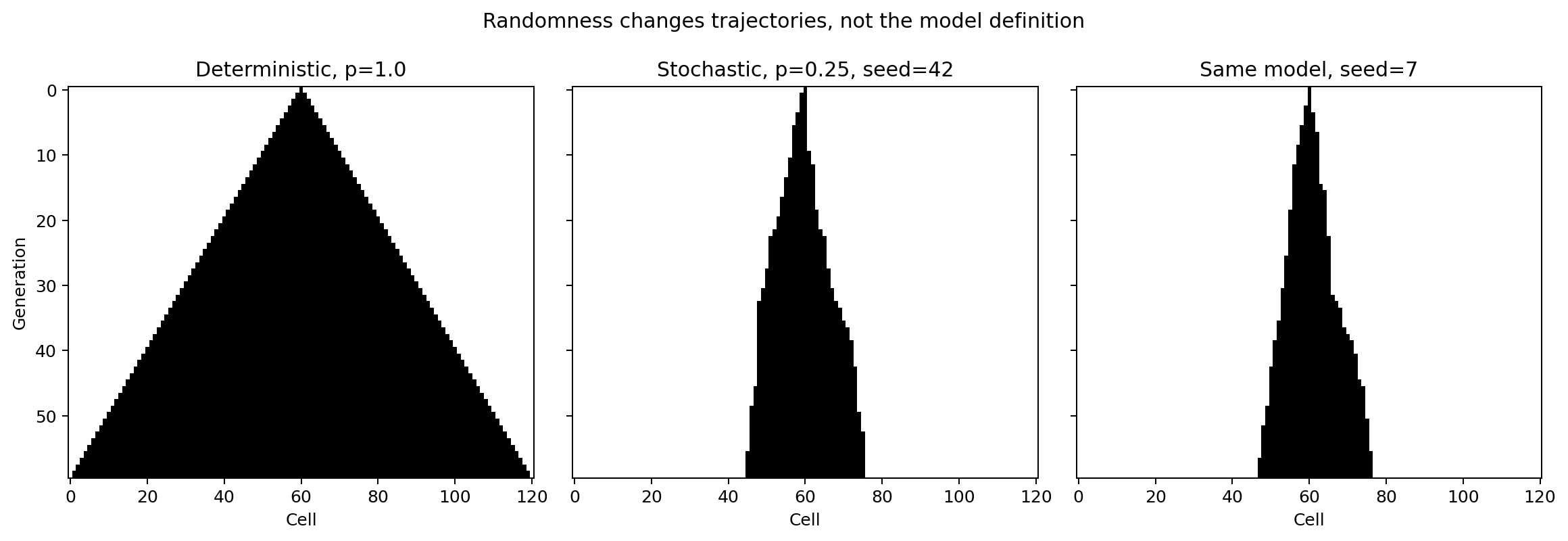
The important distinction is:

parameter p
    defines the model

seed
    selects one realization of that model

Reproducibility is part of the experiment

Use an explicit generator:

rng = np.random.default_rng(42)

Then pass it into the transition:

state = stochastic_step(state, p=0.25, rng=rng)

Running the experiment again with the same initial state, parameters and seed reproduces the same trajectory.

Changing only the seed produces another sample from the same probability model.

That gives us a useful experimental record:

initial condition
parameters
seed
steps

If any of those are missing, reproducing a stochastic result becomes harder than it needs to be.

One stochastic run is not evidence

For a deterministic automaton, one trajectory may be exactly the object we want to study.

For a stochastic model, one trajectory is usually only one sample.

Suppose we want to know how long it takes activity to occupy 80% of a line:

def run_until_fraction(
    p,
    seed,
    target=0.8,
    width=201,
    max_steps=500,
):
    rng = np.random.default_rng(seed)
    state = np.zeros(width, dtype=np.uint8)
    state[width // 2] = 1

    for step in range(max_steps):
        if state.mean() >= target:
            return step

        state = stochastic_step(state, p, rng)

    return None

Now repeat the experiment:

samples = [
    run_until_fraction(0.20, seed)
    for seed in range(200)
]

The output is no longer one answer.

It is a distribution of outcomes.

That changes the question from:

What happened?

to:

How often does each outcome happen under this model?

Measure probabilities, not anecdotes

We can estimate the probability of reaching the target within 200 steps:

def success_rate(p, runs=200):
    successes = 0

    for seed in range(runs):
        result = run_until_fraction(
            p,
            seed,
            max_steps=200,
        )
        successes += result is not None

    return successes / runs

Then sweep p:

for p in [0.05, 0.10, 0.20, 0.30, 0.50]:
    print(p, success_rate(p))

This is our first explicit move from visual exploration toward simulation experiments.

A useful stochastic result should normally report:

what was varied
what was held constant
how many realizations were run
what statistic was measured

Randomness can enter the model in different places

These are not equivalent:

Independent noise

activate = rng.random() < p

Neighborhood-conditioned probability

activate = (
    active_neighbors >= 2
    and rng.random() < p
)

State-dependent probability

p = min(1.0, 0.1 * active_neighbors)
activate = rng.random() < p

The random number generator is the same.

The causal model is different.

That distinction becomes important in the forest-fire model next, where a tree can ignite because of a burning neighbor or because of a separate spontaneous-ignition mechanism.

Vectorize the random field

On a 2D grid, generate one random field per generation:

random_field = rng.random(grid.shape)

Then combine it with deterministic eligibility:

eligible = neighbor_count(grid) >= 3
born = eligible & (random_field < 0.20)

The transition becomes:

local condition
      +
random field
      =
sampled transition mask

This is both faster and easier to inspect than hiding random draws inside deeply nested loops.

Randomness does not remove causality

If two forest-fire runs differ, we should still be able to identify the ingredients:

initial tree layout
ignition rule
spread rule
wind or directional bias
random seed

Randomness represents variation inside a defined mechanism.

It should not be used to conceal an undefined mechanism.

One idea to keep

A stochastic cellular automaton is not a deterministic automaton with noise sprinkled on top.

It is a model whose transition law includes probability.

That gives us a stronger experimental discipline:

Hold the model fixed, vary the random realization, and measure the distribution of outcomes.

In the next chapter we will use that discipline to build a forest-fire model where local ignition and fuel connectivity determine how far fire can spread.