05: So We Built the Wrong Thing on Purpose
Before trusting our own tests, we built a deliberately simple decoy and attacked it with them. Visible form wandered, heavy positional damage failed to separate cleanly from ordinary variation, and every exact relationship could be replaced without producing a reliably larger macrostate shift than the control's own variation.
The previous chapter ended with a specification: known rules, controlled interventions, one mechanism varied at a time, a history we can follow. That is the laboratory we will eventually need, and building it is most of the work still ahead.
Before building it, there is a cheaper question: are our tests any good?
That is not an idle worry. The last chapter produced the first positive result in this book — a bounded one, but a real one. Structural recurrence intersected with causal ancestry, and a causal claim survived a test we had not designed to make it pass.
Which is exactly the moment at which standards slip. Once one exciting claim has passed a test, the next exciting claim arrives with that test’s reputation already attached to it. The instrument acquires authority it has not separately earned, and it becomes easier to overlook when it reads high.
The standard laboratory response is to challenge the instrument with something that should not support the interpretation you care about.
So we spent this chapter building a system we did not believe in, and attacking it with our own evidence. It passed more of those tests than it had any right to. Violent positional damage did not reliably push it outside its measured regime. Nor did replacing every exact relationship in the system. On the way it produced one beautiful false result that we came close to believing.
None of that tells us the swarm is alive. It tells us which of our tests were cheap.
The Decoy
In experimental biology the move is routine. Alongside the sample you care about you run a negative control: a preparation in which the target condition is independently expected to be absent, processed through the same assay. If it comes back positive, you have learned something important about the assay. The same logic has been adapted in observational epidemiology to detect confounding and bias.[1]
We cannot construct that kind of negative control for digital life. We do not possess an independent test proving that a computational system is not alive.
But we can borrow the logic. We can build a deliberately simple system whose striking appearances arise from explicit local rules, then ask whether the evidence we were tempted to treat as discriminating can distinguish it.
So we built a decoy.
It is a swarm of particles. Each particle has a position and a velocity, one designated friend and one designated enemy. Friends attract. Enemies repel. A weak pull toward the centre keeps the world bounded, and a weak soft-core repulsion stops pathological collapse. That is the entire system. The specific inspiration was Simon Woods’ friend-and-enemy particle model, in which each particle moves toward one designated particle and away from another.[2] Nothing in our implementation represented a flock, a ring, a vortex, an organism, a body, a boundary, an individual, a population, reproduction or life.
Simple local rules producing coherent macroscopic order is not a new observation. Reynolds showed it in distributed flocking; Vicsek and colleagues found collective order in self-propelled particles.[3][4]
The status of the swarm needs to stay precise. We are not claiming to have proven that it is not alive. We have no procedure that would establish that, and inventing one for a case we already have an opinion about would violate the method of this book. Its role is narrower.
If a deliberately simple, fully specified decoy can exhibit a property we intended to treat as evidence of digital life, then that property cannot, by itself, distinguish the systems we care about from the decoy.
The swarm is therefore not a negative control for life. It is an adversarial calibration system for our evidence.
We built it to expose tests that were too easy to pass.
The first test was persistence.
Four Branches
We ran the swarm until it produced visible large-scale organization, then took one evolved state and split it into four identical branches: a control, material damage, organizational damage, and identity-label replacement.
Material damage displaced 30% of the particles violently while leaving every friend-and-enemy relationship intact. If persistence belonged to one particular visible arrangement of matter, this should hurt.
Organizational damage did the reverse. Positions and velocities were left exactly where they were while 30% of the friend-and-enemy relationships were rewired. If persistence required the exact relationship graph, this should hurt more.
Identity-label replacement was the strange one. Every particle carried an identity label with no causal role — nothing in the update law read it — and we progressively replaced those labels until none of the originals remained. This was not component replacement; the same dynamical particles, positions and velocities continued through the run. The intervention tested the measurement rather than the system. If changing a causally inert bookkeeping label changed our persistence score, then the score was secretly encoding nominal identity.
It did not. The branch tracked the untouched control while the original labels disappeared.
Our persistence measurement did not depend on preservation of causally inert identity labels.
That establishes almost nothing about the swarm. It tells us only that the measurement was not secretly treating a bookkeeping label as persistence.
Then the longer runs exposed a problem the short runs had hidden.
The Control Would Not Stay Still
The first runs were encouraging in the way that should always be suspicious. Damaged branches appeared to return toward a recognizable macroscopic form.
Then we ran it longer. Over a longer window the untouched control also travelled far from the reference configuration — the very state against which we had been scoring everybody else’s recovery.
For a while this looked like the experiment failing.
It was the experiment working. It had found an assumption we had never declared, never justified and never noticed making:
We had defined persistence as return to one preferred picture.
Nothing licensed that. The control did not return to its own picture either, and the control was not damaged. A definition of persistence that an undamaged system fails is not a strict definition. It is a broken one.
So the question changed. We had been asking whether the same picture came back.
Why should persistence require that?
Persistence Might Not Be a Shape
We stopped measuring distance from a privileged configuration. Instead we described each state by nineteen macroscopic features — size, elongation, speed, and a set of distance statistics — and asked a different question.
The new question was whether the system stayed inside its characteristic range of macroscopic states rather than returning to one particular picture.
That question needs a baseline, because the control moves around by itself. So before damaging anything we measured how much. We cut the untouched run into time blocks and asked how far apart those blocks were. That gave us a number for how much the system changes when nothing is done to it at all.
We will call that baseline ordinary variation. From here on, every intervention is judged against it: did the damaged swarm move farther than the untouched swarm normally moves by itself?
The same blocks answered a second question. Was the control slowly wandering somewhere new? If it were, the first and last blocks should sit much farther apart than neighbouring blocks do.
median distance, adjacent blocks     2.397

median distance, first to last       2.284

ratio                                0.953 ×
They did not: the pictures changed radically, while the statistical regime showed no corresponding cumulative drift across the observed window. OK
same visible state
≠
same dynamical regime
What our measurement could now treat as persistent was no longer a shape. It was a region of macroscopic states through which the system moves.
The exact feature list and calculations are in the Experimental Note. The two numbers above answer only one question: is the control progressively drifting somewhere new? The intervention results below use the separate ordinary-variation baseline.
Material Damage Disappears Into Ordinary Variation
Throwing 30% of the particles violently out of position produced a median shift of:
0.622 × ordinary variation
One of eight independent runs exceeded ordinary variation. None exceeded twice it.
Displacing 30% of the particles did not produce a long-run macrostate shift reliably larger, by this measurement, than the control’s ordinary variation.
That is different from saying the shape recovered. The shape did not need to return. Under this measurement, the damaged branch never separated reliably from variation the untouched swarm produced by itself.
The Result We Wanted Failed
Now the interesting branch, and the expectation behind it was not unreasonable. The friend-and-enemy assignments participate directly in the dynamics; attraction and repulsion between those pairs help generate every trajectory in the system. Rewiring 30% of them attacks causal structure while initially leaving positions and velocities untouched.
And the effect was larger:
mean distance from control

material damage          1.84

organizational damage    2.72
Organizational damage looked worse than material damage. That was exactly the result we wanted.
Unfortunately, it was not the test we had declared. The declared comparison was against the swarm’s own ordinary variation, and by that standard the apparent separation no longer held cleanly:
median      0.766 × ordinary variation

mean        0.949 ×
Two of eight runs exceeded ordinary variation. One exceeded twice it.
So the attractive sentence died — visible material can be disrupted, but persistence lives in the relationship graph. Nearly a third of the exact relationship assignments had been replaced, and the resulting macrostate distributions still did not reliably separate from ordinary variation under our measurement.
That was not the result we had hoped to find, which is precisely why the predeclared comparison was useful.
We Had Located Persistence Too Early
The pattern was becoming hard to miss. One privileged visible configuration had already failed. Thirty-percent positional damage had failed to produce a reliable departure. Now substantial exact relationship identity looked too specific as well.
| Candidate location of persistence | What the experiment showed |
|---|---|
| Identity labels | Not used by the measurement |
| Particular visible configuration | Not fixed |
| Exact positions | 30% displacement produced no reliable regime departure |
| Exact relationships | 30% edge replacement produced no reliable regime departure |
| Measured dynamical regime | Persistent so far |
There are many available explanations for that last line, and they are not equivalent. We do not get to pick one because it sounds good. What the experiment had earned was a question, not an answer:
How much of the exact relationship graph can be replaced before the measured dynamical regime changes?
That question is measurable, so we measured it.
So We Swept the Graph
For each of eight seeds, we cloned the same evolved swarm and rewired 0%, 10%, 20% and onward to 100% of its exact relationships. Everything else stayed fixed. Only the amount of rewiring changed.
Before looking at any of it, we decided what would count as a break. A dose would qualify as regime-breaking only if:
median normalized shift > 1.0

AND

at least 75% of replicates exceed ordinary variation
Declaring that in advance is a defence against one of the most ordinary forms of self-deception in experimental work: choosing, after seeing the data, which analysis counts as the analysis.[5]
So we froze it, and ran the sweep.
If the graph really carried the regime, we expected a simple pattern: more rewiring, more departure.
One dose passed.
Fifty Percent Looked Like a Threshold
At 50% rewiring:
median normalized shift                 1.430

fraction above ordinary variation       0.75

fraction above 2 × ordinary variation   0.375
Both clauses were satisfied. The metadata recorded a first operational break dose of 50%.
It is worth sitting with how good that sentence would have looked. If we had tested only that dose — and testing one intermediate dose is an entirely reasonable-sounding experiment — we could have reported the organizational breaking point of the system, with a pre-declared criterion standing behind it. It would have been the most quotable result in the chapter.
Two things should have slowed us down even then.
First, the criterion was met exactly at its boundary: six of eight replicates exceeded ordinary variation, and the rule required six. One run moving the other way would have changed the classification. Pre-declaration makes the threshold honest; it does not make the result robust.
The second problem was simpler: we had nine other doses.
Then We Looked at the Rest of the Curve
If rewiring were destroying whatever holds the regime together, the effect should grow as more of the graph disappears — and once the regime breaks, stronger damage should not make the effect vanish.
Here is what actually happened.
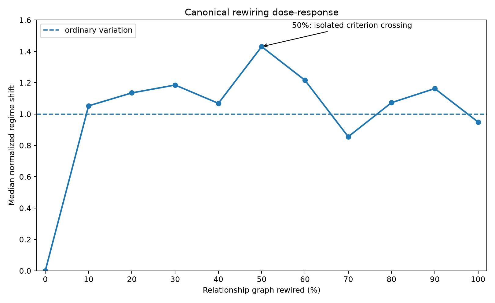
The curve is not cleanly below baseline either. Several doses produce shifts of roughly one unit of ordinary variation or more, so the data does not support the stronger claim that rewiring has no effect.
What they fail to show is a dose-response.
The sweep does not identify a monotonic graph-destruction threshold.
The isolated criterion crossing at 50% should not be promoted into a mechanistic claim, because stronger interventions do not preserve the effect.
One caution: the 30% value here is not directly comparable with the earlier 30% result because the two experiments normalize against different control baselines. Compare doses within this sweep; the construction is in the Experimental Note.
Freezing a criterion in advance protects against one specific failure: choosing the test after seeing the answer. It does not protect against another: treating a single crossing of that criterion as though it described a mechanism.
A pre-declared threshold can tell you that one result crossed a line. It cannot tell you that the system underwent a transition. For that, the whole intervention series matters, and here the series does not support one.
Every Relationship Replaced
Which leaves the strongest intervention.
At 100% rewiring, not one original friend-or-enemy assignment remained. Exact graph similarity fell from 1.0 at zero rewiring to 0.0 at complete rewiring — a manipulation check rather than a finding, since the arithmetic of the intervention fixes it. It confirms that the intervention did what it claimed.
The median normalized macrostate shift was:
0.949 × ordinary variation
Four of eight replicates exceeded ordinary variation. None exceeded twice it.
Every exact relationship in the swarm had been replaced, yet the measured long-run departure still fell within ordinary variation.
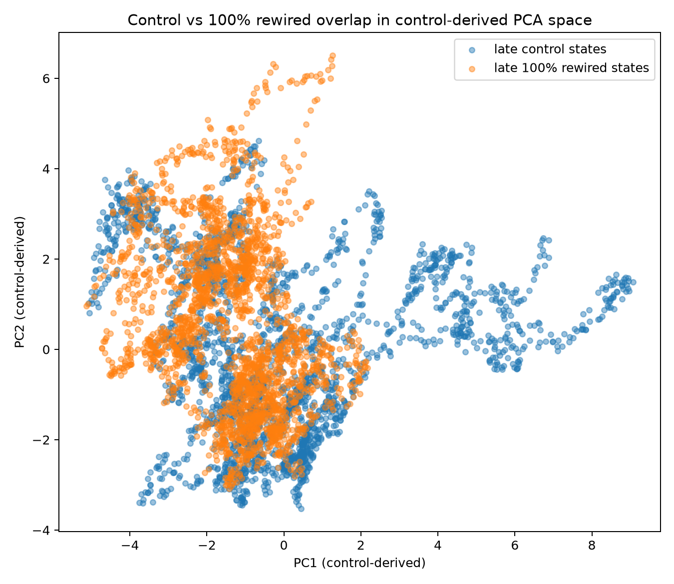
In this configuration and under this macrostate measurement, complete replacement of every exact friend-and-enemy relationship did not produce a long-run macrostate shift reliably larger than the control’s ordinary variation.
What the Result Actually Says
It does not mean relationships are irrelevant, and the difference matters.
We destroyed which particle was linked to which. The rule that builds a friend-and-enemy network remained unchanged. Even at 100% rewiring, every particle still had exactly one friend and one enemy; the attraction and repulsion rules, interaction strengths and microscopic update law were preserved.
destroyed:   which specific particle was linked to which

preserved:   the interaction law and the form of the network
So the result is narrower than relationships do not matter.
Under this measurement, replacing every original relationship was still compatible with the same measured regime. More precisely:
Exact edge identity was not required for persistence of the measured dynamical regime under this configuration.
Whatever supports that persistence is therefore not tied to preserving particular edges. It may lie in coarser graph structure, in the interaction law, or in some combination of the two.
This experiment does not separate those possibilities. They remain open questions for a different intervention.
The result suggests obvious next experiments. We have not run them.
Why It Was Worth Building the Wrong Thing
We built the swarm to expose evidence that was too easy to pass, and it did.
It looked organized. It tolerated heavy positional damage. Its visible form wandered while its measured regime remained bounded. Even complete replacement of its exact relationship graph failed to produce a reliably larger long-run departure than ordinary variation.
None of those properties, by itself, distinguishes our candidate systems from a deliberately simple system built to generate complex collective behaviour. Robustness therefore remains a real phenomenon, but it becomes weaker evidence for digital life.
This sharpens the earlier results rather than erasing them. Physarum still underwent real population turnover, but robustness alone now tells us less than it appeared to. Causal branching reproduction survives the comparison better: this swarm has no operational descendant relation and cannot counterfeit that result.
The value of the decoy is that it raises the evidential bar.
From here on, any property we propose as evidence has to discriminate against a system built specifically to counterfeit it.
We still do not know what carries persistence. We now know several things that do not.
Experimental Note
The swarm results come from one implementation.
Shorthand. Ordinary variation is the chapter’s shorthand for ordinary control self-variation. Within each experiment, it is the median energy distance across the specified blocks of that seed’s control trajectory. Normalized intervention shifts are expressed in units of that baseline.
Configuration. The four-branch damage study and the later rewiring sweep share a microscopic configuration: 256 particles, 10,000 burn-in steps, 12,000 post-intervention steps, sampling every 20 steps, and eight independent seeds. Every branch for a seed was cloned from one common post-burn-in checkpoint. Burn-in is a settling period only; no claim is made that a stationary state was reached.
Macrostate. The macrostate is a nineteen-feature vector: log radius of gyration, log anisotropy, mean speed, and quantiles of radial distance, pairwise distance, friend distance and enemy distance. All distances except radius of gyration itself are expressed relative to that radius, so the description is scale-relative by construction. The feature representation contains no particle identity label and no node-identity feature. The metric therefore cannot score persistence merely by following nominal identity, and exact relationship assignments are free to change without being encoded directly as features.
Distance and normalization. Feature vectors are z-scored using a standardizer fit only on pooled control states. Distribution distance is the multivariate energy distance between the late halves of two trajectories, computed on deterministically subsampled points. Normalized shift is that distance divided by the control’s own internal spread.
Two denominators. The four-branch study and the rewiring sweep construct that denominator differently: the former uses the late half of the control cut into three blocks; the latter uses the full control trajectory cut into six. Ratios are therefore comparable within each experiment and not numerically across the two. This is why the 30% organizational-damage ratio in the four-branch study and the 30% row of the sweep are not replications of one another. The adjacent-block and first-to-last values reported in the chapter are a separate diagnostic for cumulative drift and are not the denominator used for intervention ratios.
Preserved under 100% rewiring. Every particle still had one friend and one enemy; the attraction rule, the repulsion rule, the interaction strengths, the particle count, the class of network and the microscopic update law were all unchanged. The intervention destroyed edge identity, not network form or interaction law.
Manipulation check. Graph-similarity values are fixed by the intervention arithmetic rather than being empirical outcomes: the rewiring operation forbids reassignment to the previous target, so exact similarity is determined by dose. Similarity fell from 1.0 at 0% rewiring to 0.0 at 100% across the sweep.
Pre-declaration. The break criterion — median normalized shift above 1.0 and at least 75% of replicates above ordinary variation — was frozen in the configuration before the sweep was inspected.
Bounds on the claims. Every claim about regime persistence in this chapter is conditional on the nineteen-feature representation, the chosen normalization and the energy-distance metric. A different representation could separate branches that this one does not. Failure to detect a departure here is not evidence that the underlying states were identical or that no causal change occurred.
Sample size. Eight replicates per dose is a small sample. The dose-response curve supports an absence of detected monotonic dose-dependence under this analysis; it should not be read as a precise estimate of effect size. Bootstrap confidence intervals on each dose’s median ratio belong with the per-dose results in the appendix.
Full parameters, feature definitions, standardizer construction, intervention protocols, per-seed results and discarded runs are provided in the appendix.
References
[1] Lipsitch, M., Tchetgen Tchetgen, E. & Cohen, T. Negative Controls: A Tool for Detecting Confounding and Bias in Observational Studies. Epidemiology 21(3), 383–388 (2010). doi:10.1097/EDE.0b013e3181d61eeb
[2] Woods, S. Dancing with friends and enemies: boids’ swarm intelligence. Wolfram Community (2012).
[3] Reynolds, C. W. Flocks, Herds, and Schools: A Distributed Behavioral Model. Computer Graphics 21(4), 25–34 (1987). doi:10.1145/37402.37406
[4] Vicsek, T., Czirók, A., Ben-Jacob, E., Cohen, I. & Shochet, O. Novel Type of Phase Transition in a System of Self-Driven Particles. Physical Review Letters 75(6), 1226–1229 (1995). doi:10.1103/PhysRevLett.75.1226
[5] Simmons, J. P., Nelson, L. D. & Simonsohn, U. False-Positive Psychology: Undisclosed Flexibility in Data Collection and Analysis Allows Presenting Anything as Significant. Psychological Science 22(11), 1359–1366 (2011). doi:10.1177/0956797611417632