08: The Crystal Gets a Past
A saved state can continue the Digital Crystal exactly, an event history can reconstruct how it formed, and a single received bit can redirect its future. None of that is memory yet.
At the end of the last chapter the Digital Crystal could tell us something about the world that formed it. Hide the forcing process, show only the final shape, and the family of that process could be recovered well above chance. Then we asked a harder question.
What happened first?
We took exactly the same environmental values and rearranged them in time. Smooth. Bursting. Periodic. Alternating. Random. The final morphology could not reliably tell them apart.
SAME VALUES
+
DIFFERENT ORDER
↓
TEMPORAL ORGANIZATION
NOT RECOVERED UNDER THE TESTED READOUT
The crystal had accumulated consequences of its past. Its final morphology had not given us a reliable readout of temporal order. So the previous chapter ended with an instruction rather than a conclusion: give the process a way to keep what happened. That sounds like a storage problem. But storing more information would be easy. The difficult question is deciding which information actually constitutes a computational past. Before we build memory, we need to discover what a future can still depend on. So the question for this chapter is deliberately small:
What must a computational process preserve before its past can become available to its future?
Notice that this is not the same as asking how to build memory. We have not earned that word, and we do not yet know what it would mean here. What we can do is take the words that ordinary language collapses into one — state, history, record, influence, signal, message, memory — and pull them apart until each of them names a different computational property. The experiments will force those words apart.
The Present Is Not the Past
The Digital Crystal already has a present. At any moment its occupied set contains the cells that currently exist, and every one of those cells exists because of something that happened earlier. So the past clearly mattered. But the previous chapter taught us a distinction that is easy to state and easy to forget:
Past contributed to present does not imply present contains a recoverable record of the past.
A footprint exists because someone walked there. The footprint is not the walk. Likewise, the crystal’s current shape contains consequences of earlier events without necessarily preserving the sequence of those events. A consequence of the past is not yet a record of the past. Two ideas are tangled together here. This chapter pulls them apart:
STATE
→ what must I know to continue from here?

HISTORY
→ what must I know to reconstruct how I got here?
Those are different questions. There is no guarantee that the same information answers both. There is no guarantee that either of them is visible in the picture. We can test all of that.
Stop It
Begin with state, because state has an operational definition available:
A state representation is sufficient if it contains enough information to continue the process faithfully from here.
That wording is careful. We are not claiming to know the smallest possible state of a Digital Crystal. We are asking whether a particular stored representation is sufficient — a question an experiment can answer. Take the frozen Digital Crystal from the previous chapter and run it for 96 steps. At step 48, save everything we currently believe the process needs in order to continue:
occupied cells
birth-time metadata
current timestep
current signal position
random-number-generator state
model parameters
Not a screenshot. Not merely the visible crystal. Save the process, destroy the running instance, reconstruct it from the saved state, and continue.
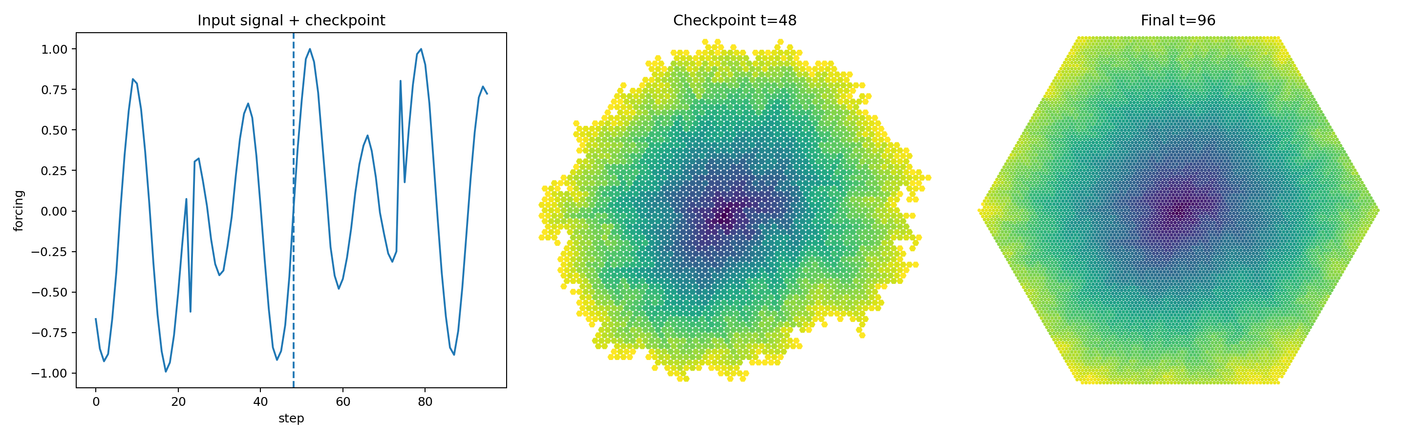
The continuous reference trajectory. The midpoint checkpoint will be restored, damaged and replayed in the experiments that follow.
Then demand something much stronger than visual similarity. If the checkpoint is sufficient, the restored process should not resemble the uninterrupted one. It should reproduce it:
the same cells
the same attachment decisions
the same population trajectory
the same final process state
Exact continuation, or the representation was incomplete.
Restore It
Save the process at step 48. Destroy the running instance. Load the checkpoint from storage and continue to step 96.
exact final morphology            True
exact final process state         True
population trajectory identical   True
attachment trajectory identical   True
symmetric-difference cells        0
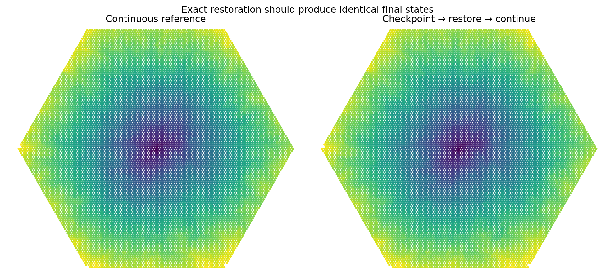
Continuous execution and checkpoint → restore → continue produce the same trajectory, cell for cell.
Repeated across 30 independent runs, all 30 restores continued exactly. So we have earned the first claim of the chapter:
The stored checkpoint representation is sufficient for exact continuation of the stochastic process.
Note the limit of the claim. The experiment establishes that this representation is sufficient for exact continuation; it does not establish that it is minimal. There is something distinctly computational about the result. We stopped the process, recorded its state, destroyed the running instance, restored it, and recovered the same future it would otherwise have followed — cell for cell, decision for decision. This is an affordance of the computational substrate rather than a biological mechanism reproduced in software.
What the Picture Cannot Show
Now damage the checkpoint deliberately, one component at a time, and see which damage the future notices. Every variant gets exactly 48 continuation updates, so that moving the environmental cursor does not accidentally shorten the experiment. Throughout this section, symmetric-difference cells means occupied positions present in one final crystal but not the other.
Remove the random state. Same morphology, same birth metadata, same timestep, same signal position, different stochastic continuation state:
symmetric-difference cells 28
Small, but not zero. Exact continuation fails.
Move the environmental cursor. Same morphology, same random-number-generator (RNG) state, same number of remaining updates, but the process now sits at position 45 in the signal instead of 48:
symmetric-difference cells 27
Replace the birth times. Keep occupied cells, RNG state, signal cursor and timestep; scramble the metadata recording when each cell appeared:
symmetric-difference cells 0
Exact. The growth rule never consults birth times when deciding the next attachment, so they can be wrong without the geometry noticing.
Save only the picture. Preserve the visible occupied structure and reconstruct everything else incorrectly:
symmetric-difference cells 30
The visible shape at the checkpoint was identical. The future was not.
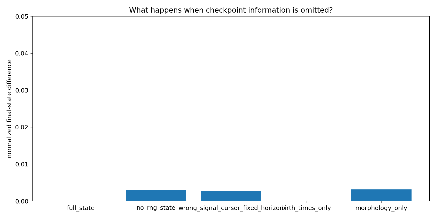
Visible morphology is insufficient for exact continuation. Stochastic state and environmental position affect future growth; birth-time metadata does not affect the occupied-set continuation.
Two distinctions fall out immediately.
The first:
VISIBLE FORM
≠
EXECUTABLE STATE
Two Digital Crystals can be pixel-for-pixel identical and still be in different states, because the information that decides their futures is not all information that appears in the rendering. Anything looking at the picture — including us, including any classifier we train — is looking at a projection of the state, not the state.
The second is subtler:
HISTORICAL INFORMATION
≠
CAUSALLY ACTIVE CONTINUATION STATE
Birth times are real information about the past. They are stored and accurate, but the future is entirely indifferent to them. Historical information can therefore exist inside a process without contributing to what the process does next. That distinction will matter when we ask whether stored history has causal leverage.
So the useful operational idea is:
Continuation state is the information required to reproduce the process’s future under the same later conditions.
Not whatever information happens to exist in our data structures, and not whatever information sounds philosophically important.
Replay What Happened
The checkpoint answers where are we now. It says nothing about how did we get here. You can restore the system from a checkpoint, but that does not recover the path by which it arrived there. For that we record events. At each growth step we store the step index, the input value, the cells that appeared, the resulting population and a hash of the resulting morphology:
t1 → these cells attached
t2 → these cells attached
t3 → these cells attached
...
Then we test the record the way we tested the checkpoint — by demanding that it be sufficient for something. Do not rerun the growth rule. Instead take the recorded event stream, apply each step’s additions to a bare lattice, recompute the morphology hash, and compare it against the hash recorded at the time. Across 96 recorded steps:
96 / 96 morphology hashes match
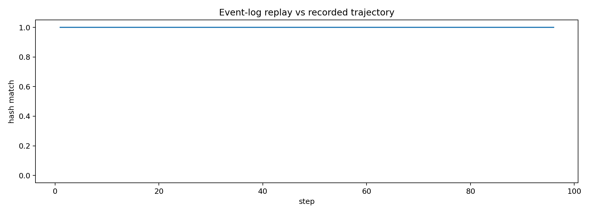
The event history reconstructs the recorded morphology trajectory exactly: 96 matching hashes out of 96.
The second claim of the chapter:
The explicit event history is sufficient to reconstruct the exact recorded morphology trajectory.
And now the two mechanisms can be compared, which is the point of having built both. The event history does not contain the historical stochastic state. Reconstruct the geometry from the log, hand it forward without the correct RNG continuation state, and exact continuation fails — by the same margin as the morphology-only checkpoint, because that is effectively what it is. So the two representations answer different questions:
CHECKPOINT
→ sufficient for exact continuation

EVENT HISTORY
→ sufficient for exact reconstruction of recorded morphology
or more compactly:
STATE
→ FUTURE

HISTORY
→ PAST
They overlap. They are not interchangeable. A process can preserve enough information to reconstruct its past without preserving what it would need to regenerate its exact future from that reconstruction — and, as the birth-time result showed, the reverse holds too. Notice what we have not done. We have not invented a memory organ or searched for a special geometric region containing the past. We used computational affordances — checkpointing, event recording and replay — to separate continuation from reconstruction. That is useful instrumentation. It is not yet a property of the crystal itself.
Whose Past Is This?
Here is the moment to be careful, because we have just built an impressive amount of machinery and none of it belongs to the crystal. We have checkpointing, serialization, event logs, replay, restore, branching. The Digital Crystal has none of these. It does not read the log. It does not ask what happened earlier. Its attachment rule contains no term that consults a stored record, and if we deleted the entire database mid-run the growth would proceed exactly as before.
A system having a recorded history is not the same thing as the system possessing that history.
The distinction to keep is between:
WE CAN RECOVER ITS PAST
and:
ITS PAST IS CAUSALLY AVAILABLE TO IT
Those are different claims, and only the first is supported. What we have built is instrumentation. Excellent instrumentation — it will carry the next six chapters — but instrumentation is a property of the laboratory, not of the specimen. So we now have a recoverable account of the crystal’s past. That account belongs to the laboratory, not to the crystal. We can recover its past; the crystal cannot yet use it.
Fork the Future
The checkpoint has one more consequence, and it changes what kind of experiments become possible. Restore the same saved state twice. Both copies begin with identical occupied cells, timestep, signal cursor and stochastic state. Nothing whatsoever differs. Then change what happens next in one of them.
             SAME CHECKPOINT
                  |
          ┌───────┴───────┐
          |               |
     FUTURE A         FUTURE B
Here the computational substrate gives us something experimentally unusual: an exact executable branch point. From one saved state we can construct alternative futures directly rather than search the world for approximately matched cases. This is the single most valuable thing the checkpoint gives us, and everything in the second half of this chapter depends on it. The branch point gives us control, but stochasticity immediately adds a warning. Two futures can diverge even when we do not manipulate the mechanism we care about. So from this point onward, every measure of counterfactual divergence needs a stochastic baseline. That problem will become considerably more important later in the chapter.
Before There Are Messages
Now the machinery gets pointed somewhere new. Our history is made of events, and until now every event has stayed inside the experimental record. But an event does not have to remain internal. One process can emit one. Another process can receive it. The temptation is immediate and enormous: two crystals, one event, therefore communication. That word arrives carrying far more than we have earned. A sender. A receiver. A message. A channel. Meaning. Perhaps intention. We have established none of it. So we begin with something smaller than a message.
Before there are messages, there are events that can alter another process.
Call it a pulse. The Digital Crystal itself stays frozen — same lattice, same local growth rule, same dependence on a scalar environmental input. We add one coupling mechanism outside that rule: the laboratory derives a one-bit pulse from the sender’s own growth dynamics. One update later, a received pulse adds 0.65 to the receiver’s ordinary environmental forcing for that update. The sender and receiver retain independently generated external environments. So the channel does not replace the receiver’s environment. It perturbs a scalar the receiver was already using.
    flowchart LR
    S["Sender growth"] --> E["Endogenous one-bit event"]
    E --> R["Receiver forcing changes"]
    R --> P["Attachment probabilities change"]
    P --> M["Receiver morphology may diverge"]
The receiver does not get a sentence, a symbol, a sender identifier, a goal or an instruction. It gets a perturbation to a number it was already reading. That design decision is the whole point. An earlier version of this experiment had coupled auxiliary oscillators to each crystal and looked for synchronization between them — which might have produced a perfectly interesting dynamical system while leaving the growth process we actually care about almost untouched. The question that matters is whether the bit reaches the thing we are studying.
The Sender Does Not Fire on a Clock
It would be easy to generate pulses on a schedule:
if step % 10 == 0:
    send(1)
But then the timing would come from the experimenter rather than from the crystal.
Instead we derive pulses from the sender’s own growth. A simple laboratory-defined detector watches its recent attachment activity and emits a pulse when the current step is unusually active relative to that recent baseline. The precise threshold is not a property of the Digital Crystal; it is simply the mechanism we use to turn changes in the sender’s growth into a one-bit event.
The important constraint is where the event comes from. No timer and no receiver state enter the emission decision. The sender’s own changing growth determines when pulses occur, and each pulse is delivered to the receiver one update later.
At this stage the bit carries no assigned meaning. It records only that the sender crossed the experimental event threshold.
There is one practical limit on the experiment. If a crystal grows close to the edge of its finite lattice, different trajectories begin to converge on the same filled boundary. We therefore stop the runs before that boundary dominates the result. The exact detector parameters and saturation limits are recorded with the experiment.
One Bit Changes the Future
The first paired intervention looked unusually clean. Take a receiver checkpoint. Fork it. Both branches begin with the same morphology, birth metadata, stochastic state, environmental forcing, timestep and remaining horizon. Change exactly one thing: one branch receives a bit, the other does not.
    flowchart TD
    CK["Checkpoint: identical receiver state"] --> BIT1["BIT = 1"]
    CK --> BIT0["BIT = 0"]
    BIT1 --> FUT_A["Future A"]
    BIT0 --> FUT_B["Future B"]
    FUT_A --> COMP["Compare final morphology"]
    FUT_B --> COMP
This is an intervention rather than a correlation. The bit is the only deliberately changed input between the paired branches. If their outcome distributions differ, the intervention has causal effect. How large the pathwise difference should be credited to that bit will turn out to require more care. Repeated 120 times:
paired interventions              120
produced morphology divergence  95.8%
mean normalized difference     0.1633
Here, normalized difference is:
cells occupied in exactly one branch
────────────────────────────────────
cells occupied in either branch
so 0 means identical occupied sets and larger values mean greater morphological separation. Five of the 120 interventions produced no final morphological difference. That constrains the result usefully: the claim is not that every bit deterministically changes the receiver. The result is not every received bit changes the receiver. It is:
Changing one received bit, while holding receiver state, stochastic state and external forcing fixed, usually altered the receiver’s subsequent morphology.
The bit reaches the actual growth process. We have established primitive causal transmission through the imposed coupling. That is smaller than communication, and it is enough.
The Crystal Can Hear a Pulse
We have established one important fact: a bit generated by one crystal can enter another crystal and alter what the receiver subsequently becomes.
That is causal transmission.
It is not yet enough to call the process communication in the stronger sense. For that, the transmitted pattern would have to carry something about the sender that the receiver can distinguish.
So the next question is:
Does something specific about the actual sender survive transmission in a way the receiver distinguishes?
We tested that by progressively replacing features of the real sender’s pulse stream.
Does the Timing Matter?
First, keep the same number of pulses but shuffle when they occur.
For each run we measure the largest correlation between the incoming pulse stream and the receiver’s subsequent attachment activity across the declared lag window.
The real sender stream performs better than the shuffled version:
real minus shuffled       ≈ +0.294
pairwise superiority      ≈  0.980
Here, pairwise superiority is the probability that a randomly selected real-stream result exceeds a randomly selected control result, with ties counting half.
We then use an even simpler control: preserve the total number of pulses but place them at random times.
real minus random         ≈ +0.270
pairwise superiority      ≈  0.977
So the result cannot be explained merely by how many pulses the receiver receives.
The timing of the pulses matters.
That establishes more than simple pulse count, but it still does not tell us whether the receiver is responding to anything specific about this sender.
Does the Actual Sender Matter?
Now replace the real sender with another Digital Crystal of the same type.
The substitute crystal has its own independent environment and growth history. We force its pulse count to match the real sender exactly, then give its stream to the same kind of receiver.
If the real sender is transmitting something sender-specific, its stream should produce a stronger relationship with the receiver than the matched stream from this unrelated crystal.
It does not:
real minus unrelated      ≈ -0.015
pairwise superiority      ≈  0.457
There is no meaningful advantage for the actual sender.
The receiver therefore responds to temporal structure in the incoming pulses, but this experiment gives us no evidence that it can distinguish which crystal produced them.
Does the Exact Sequence Matter?
There is still another possibility. Perhaps the information lies in the exact ordering of the gaps between pulses.
So we take the real pulse stream, measure every interval between pulses, preserve that entire collection of intervals, and shuffle their order.
The surrogate therefore has:
same number of pulses
same collection of intervals
different ordering of those intervals
Again, the real stream has no meaningful advantage:
real minus surrogate      ≈ +0.010
pairwise superiority      ≈  0.473
Whatever effect we are measuring does not appear to depend on the exact chronology of those intervals.
The evidence now separates two claims that initially looked very similar:
| Claim | Result |
|---|---|
| A received pulse can alter the receiver | Supported |
| Pulse timing matters | Supported |
| Pulse count alone explains the effect | Rejected |
| The receiver distinguishes the actual sender | Not supported |
| Exact interval ordering carries a detectable sender-specific signal | Not supported |
The crystal can therefore respond to an incoming event stream without yet distinguishing its source.
Connectivity Is Not Coordination
We also asked whether this primitive transmission became more meaningful when many crystals were connected.
Six crystals arranged in a line produced source-to-node correlations that looked like propagation. But when we shuffled which upstream crystal supplied each downstream connection, almost the same pattern remained:
mean absolute real-vs-shuffled difference
≈ 0.0164
We then tested a 6 × 6 board of thirty-six locally connected crystals.
Again, the real neighbourhood structure barely outperformed a shuffled control:
real minus shuffled neighbour correlation
≈ 0.0048
These are exploratory topology tests, but their lesson is useful.
Connecting crystals gives us connectivity. It does not by itself give us evidence of coordinated collective behaviour.
The experimental ladder therefore ends here:
causal transmission
        YES
         ↓
timing-sensitive response
        YES
         ↓
sender-specific signalling
         NO
         ↓
network-level coordination
         NO
The bounded result is:
Within Digital Crystal v1, changing one received bit while holding receiver state, stochastic state and external forcing fixed can alter the receiver’s subsequent morphology. Real sender-generated pulse timing produces stronger receiver relationships than shuffled or rate-matched random timing, but it does not outperform count-matched same-class sender replay or an interval-preserving surrogate. This supports primitive causal transmission, not sender-specific signalling.
Or more simply:
The crystal can hear a pulse. It cannot yet tell who spoke.
What the Failure Was Actually Telling Us
It would be lazy to summarize that as communication failed.
Look at what the control ladder actually mapped.
The receiver is sensitive to something destroyed by shuffled and rate-matched timing controls.
But the next two controls tell us how little we know about what that something is. A count-matched same-class sender performs as well as the actual sender. So does a surrogate preserving the exact multiset of inter-pulse intervals while changing their order.
The experiment does not isolate burstiness, interval distribution, local pulse density or any other single statistic as the carrier.
What survives is narrower:
COARSE TIMING STRUCTURE
        MATTERS

ACTUAL SENDER IDENTITY
        NOT SUPPORTED

EXACT INTERVAL CHRONOLOGY
        NOT SUPPORTED
The transmission is lossy.
And it rhymes with the experiment that brought us here:
PREVIOUS CHAPTER

broad source characteristics
        RECOVERABLE

temporal organization
        NOT ESTABLISHED

THIS CHAPTER

coarse pulse-stream structure
        MATTERS

sender identity and exact chronology
        NOT ESTABLISHED
Twice now, different experiments have produced the same suggestive pattern:
coarse temporal structure survives
fine temporal identity does not
What Counts as the Same Random World?
This turned out to be more than a technical problem with random numbers. It changed the meaning of our causal experiments.
We had been treating divergence between paired stochastic trajectories as though it measured the consequence of an intervention. But that divergence also depends on how random opportunities are matched between the two worlds.
Before asking how strongly an intervention changes the future, we therefore have to define what counts as the same stochastic future.
Digital Crystal growth is stochastic. When we fork a checkpoint into a treated and an untreated branch, we hold the random-number state fixed and assume that gives us two versions of the same random world.
It does not. It gives us two versions of the same random stream.
Here is the mechanism. At each step the process builds a frontier of candidate cells, sorts it, and hands each candidate the next value from the stream. Perfectly reproducible — as long as both branches present the same candidates in the same order. But the intervention changes an attachment, which changes the frontier, which changes the sorted list. From that moment the two branches are consuming the same sequence of numbers in different places. Random value 27 lands on a different cell in each world, and every value after it is misassigned relative to its counterpart.
Imagine two identical card tables, each being dealt from an identically ordered deck. Remove one player from one table. That table does not merely lose a player: every card after the gap now lands in a different hand. Compare the two tables afterwards and you will measure an enormous difference — but much of it is not the consequence of the missing player. It is the consequence of the reshuffle you caused by removing them.
So some of the dramatic pathwise divergence in our early perturbation experiments could come from reassigned stochastic opportunities rather than from downstream amplification of the intervention itself.
The causal effect remained real.
Its apparent cascade had become suspect.
SAME RANDOM STREAM
≠
SAME RANDOM OPPORTUNITIES
The Cascade Shrinks
The fix is to key randomness to the event rather than to the sequence.
We built a second experimental runner in which each possible attachment opportunity draws its random value from a function of the seed, the absolute step and the cell coordinate. A cell at a given position at a given step then sees the same random value in both branches. If a cell exists in one branch and not the other, only that opportunity differs; a change to the frontier somewhere else no longer shifts every subsequent draw.
This is a common-random-number coupling, and it needs a clear label:
The cell-keyed runner is an experimental coupling, not a replacement for the canonical Digital Crystal.
The canonical model remains the sequential stochastic process introduced in The Digital Crystal. The keyed runner exists only to define a cleaner paired counterfactual — and before using it, we had to check we had not quietly built a different crystal. Across 96 runs per implementation, the omnibus morphology comparison between the two found no evidence of a gross distributional discrepancy (p ≈ 0.922), and four predeclared practical-compatibility margins all passed. That is not proof that the two processes are mathematically identical. It is enough to use the instrument for the experiment it was declared for.
Then repeat the pulse experiment under both couplings and compare like with like.
For scale, define independent divergence as the drift produced when two continuations start from the same experimental context but use independently reseeded stochastic futures.
Now ask how large the pulse-induced paired divergence is relative to that reference:
sequential RNG coupling                              Right OK ≈ 87% of independent-divergence scale
cell-keyed common-random-numbers (CRN) coupling      ≈ 11% of independent-divergence scale
    flowchart TD
    A1["Pulse branch, sequential RNG"] --> B1["Frontier changes"]
    B1 --> C1["Stream misaligns"]
    C1 --> D1["Large apparent divergence"]
    A2["Pulse branch, cell-keyed CRN"] --> B2["Frontier changes"]
    B2 --> C2["Same cell sees same draw"]
    C2 --> D2["Small residual divergence"]
    D1 --> E["Much of the cascade was coupling artifact"]
    D2 --> F["Causal effect is real and much smaller"]
The pulse did not stop mattering. The intervention remains causal under both couplings. What collapsed was the apparent explosion of consequences that followed it.
This is not a footnote about random-number generators. It changes what a counterfactual trajectory is in a stochastic computational system:
CAUSAL EFFECT
≠
COUPLING-INVARIANT PATHWISE DIVERGENCE
This forces another separation.
difference between outcome distributions
≠
paired difference under a declared stochastic coupling
≠
distance between two particular trajectories
A related correction belongs here too. Before the coupling was fixed, four-pulse sequences appeared to produce a response that was substantially different from the sum of the individually measured pulse responses — an attractive result, since nonlinear integration of input history would be a genuinely interesting property. After the coupling fix we added a measurement-noise floor: how large a mean feature difference appears when you compare two finite samples drawn from the same unperturbed population? The floor came out around 0.045. The superposition residual was around 0.007.
The effect was several times smaller than our ability to see it. So:
OBSERVED DISCREPANCY
≠
RESOLVED MECHANISTIC NONLINEARITY
Within the resolution of this experiment, the multi-pulse response stayed compatible with the sum of the isolated responses. The discrepancy existed.
The experiment could not resolve it as a mechanistic effect.
Two Histories
Now, finally, the question the chapter has been walking toward.
We know a pulse changes the future. Does the arrangement of pulses leave a trace?
The naive comparison is too easy. Compare 11110000 against 10010010 and a classifier might succeed merely because one crystal was perturbed more recently than the other. That would be recency detection, not history retention.
So the confirmatory experiment used two codewords built to remove the cheap cues:
A = 11100001      pulses at {0, 1, 2, 7}
B = 10001101      pulses at {0, 4, 5, 7}
Same number of pulses. Same first pulse. Same last pulse. Only the interior arrangement differs.
The confirmatory experiment was frozen before the result was inspected: codewords, stochastic coupling, primary endpoint and primary morphology measurement.
The first measurement occurred immediately after the final pulse. Further measurements followed one, two and four updates later.
The primary endpoint was frozen at step 8, using a regularized paired multivariate statistic over nine angular morphology features. A wider 24-feature measurement and the later endpoints were secondary.
They were recorded.
They were not allowed to rescue the primary experiment.
Otherwise every negative result becomes permission to keep searching until some alternative statistic succeeds.
Forty-eight independently generated receiver checkpoints.
Does temporal arrangement leave a stable, reproducible morphological signature across independently generated receivers?
Different Futures, No Stable Signature
The two histories did not produce identical crystals. Immediately after the final pulse, the average normalized symmetric difference between paired futures was about:
0.053 [0.048, 0.059]
So the interior arrangement of the pulses had real causal consequences. Rearranging when the bits arrived changed what the receiver became.
The population-level test asked for something stronger, and found no evidence for it.
primary angular test (9 features)      p = 0.7366

secondary test (24 features)           p = 0.9320
The predeclared primary statistic showed no evidence of a stable history signature, and the wider secondary measurement did not recover one either.
The experiment passed its implementation, preflight and coupling checks. What failed was the prediction: neither the primary nor the secondary measurement recovered a stable population-level history signature.
The bounded result is:
Under the frozen protocol, changing the interior timing of four pulses while holding pulse count, onset and offset fixed did not yield evidence of a reproducible population-level morphology signature detectable by the predeclared angular measurement at the primary endpoint.
That is a clean negative result for the predeclared test.
It is not evidence that temporal arrangement can never matter, and it does not mean the two histories had no consequences.
DIFFERENT HISTORY → DIFFERENT PARTICULAR FUTURE
SUPPORTED

DIFFERENT HISTORY → STABLE POPULATION-LEVEL SIGNATURE
NOT SUPPORTED UNDER THE PREDECLARED TEST
There is a tempting sentence here: the crystal forgot the sequence. We cannot say that. Forgetting presupposes something like memory to lose. What we can say is stranger and more useful:
The past can change the present without leaving an obvious trace of how it did so.
A Past With Consequences
Put the three experiments side by side and a hierarchy appears that was not visible from any one of them.
CAUSAL CONSEQUENCE
        ↓
PERSISTENT CONSEQUENCE
        ↓
SYSTEMATIC SIGNATURE
        ↓
RECOVERABLE INFORMATION
Every arrow is a new empirical claim.
The Crystal has crossed the first threshold repeatedly.
The experiments in this chapter show why none of the later thresholds follows automatically.
That is the shape of the chapter, and it is worth being clear that this is a chapter with a great deal in it. Several strong interpretations died. The phenomena underneath them did not.
The strongest surviving progression is:
complete state
→ exact continuation

recorded events
→ exact reconstruction

earlier intervention
→ later causal consequence

different histories
→ different particular futures
Three distinctions now matter more than the rest:
VISIBLE FORM
≠
EXECUTABLE STATE

RECORDED PAST
≠
CAUSALLY AVAILABLE PAST

CAUSAL CONSEQUENCE
≠
MEMORY
The single sentence the chapter has earned:
The past has become causally real before it has become memory.
Experimental Note
This chapter combines three experimental layers built on the same frozen Digital Crystal v1 substrate.
The state/history experiment used a 96-update full-profile trajectory with a checkpoint at update 48. Thirty independently seeded checkpoint restores reproduced both final morphology and complete continuation state exactly. Symmetric-difference cells counts occupied positions present in exactly one of two compared states.
The signalling experiments used independently seeded sender and receiver environments. In the full profile, the endogenous pulse rule used a 12-update recent-activity window, a 0.75-standard-deviation threshold with a minimum of three attachments, one-update delivery delay and receiver coupling gain 0.65. Normalized morphology difference is occupied-set symmetric difference divided by occupied-set union. Peak message-to-growth correlation is the maximum lagged correlation between the pulse stream and receiver attachment counts over the declared lag window. Pairwise superiority is the empirical cross-sample probability that a statistic from one condition exceeds one from another, with ties weighted by one half.
The later counterfactual experiments use a separate cell-keyed common-random-number runner. It assigns random values by (seed, absolute step, cell) so corresponding cell/time opportunities receive the same draw across paired branches. This runner is an experimental coupling instrument, not a replacement for the canonical sequential-RNG Digital Crystal.
The matched-history confirmation used 48 independently generated receiver checkpoints. The two codewords contained equal pulse counts and identical first and last pulse positions. The primary endpoint and nine-feature angular measurement were frozen before the confirmatory result was inspected; later endpoints and the 24-feature measurement were secondary.
Full parameter values, raw distributions, confidence intervals, control construction, compatibility margins and reproducibility records are preserved with the accompanying experiment reports.
| Claim | Status | Evidence |
|---|---|---|
| Complete checkpoint resumes the exact trajectory | SUPPORTED | 30/30 exact restores; symmetric difference 0 |
| Visible morphology alone is sufficient continuation state | FAILED | 30-cell divergence |
| Stochastic continuation state matters for exact continuation | SUPPORTED | 28-cell divergence when removed |
| Environmental sequence position matters at fixed horizon | SUPPORTED | 27-cell divergence when shifted |
| Birth-time metadata affects occupied-set continuation | FAILED | 0 differing cells |
| Event history reconstructs the recorded morphology trajectory | SUPPORTED | 96/96 trajectory hashes |
| Event history restores historical stochastic state | NOT SUPPORTED | additions alone do not contain it |
| Checkpoint is an executable counterfactual branch point | SUPPORTED | controlled alternative continuations |
| A received one-bit event can alter receiver morphology | SUPPORTED | 120 paired interventions; 95.8% diverged |
| Real pulse timing beats shuffled and rate-matched timing | SUPPORTED | differences ≈ 0.294 and 0.270 |
| The actual sender matters more than a same-class sender | FAILED | difference -0.015; superiority 0.457 |
| Exact chronology matters beyond the same interval multiset | FAILED | difference 0.010; superiority 0.473 |
| Influence propagates specifically through chain topology | FAILED | real-vs-shuffled ≈ 0.0164 |
| Local 6×6 topology produces organized signalling | FAILED | real-vs-shuffled ≈ 0.0048 |
| Pathwise divergence depends on stochastic coupling | SUPPORTED | ≈87% sequential vs ≈11% cell-keyed |
| Multi-pulse response is nonlinear | FAILED | residual 0.007 below measurement floor 0.045 |
| Matched pulse histories produce different particular futures | SUPPORTED | normalized difference 0.053 |
| Matched pulse histories leave a population-level signature | FAILED | p = 0.7366; secondary p = 0.9320 |
| The crystal possesses or consults its recorded history | NOT CLAIMED | no mechanism consults the record |
| The crystal remembers, learns, communicates or coordinates | NOT CLAIMED | evidence insufficient |
Put the Past Into the Material
So where, exactly, is the crystal’s past?
Not in our checkpoint — that belongs to the laboratory. Not in our event log — the growth rule never reads it. Not in the morphology, which turned out to be a projection of the state rather than the state itself, and which could not be made to give up the arrangement of the pulses that shaped it.
And yet the past is unmistakably doing something.
A pulse changes an attachment. That attachment changes the frontier. The changed frontier alters later opportunities. The process follows a different trajectory.
event
↓
local consequence
↓
changed possibility
↓
later consequence
Which suggests the next experiment, and it is smaller than memory and more concrete than history.
So far, an occupied Crystal cell has almost no internal state.
It cannot be changed by experience and remain changed afterwards.
It cannot carry a persistent local distinction such as:
this happened here
≠
this did not happen here
Any detailed record we currently possess lives outside the material:
checkpoint
database
event log
What if experience changed the material itself?
Change the material.
Then remove the event that changed it.
If the material difference persists, remains accessible to later computation, and changes what the process does next, then the past will have acquired something it has not had anywhere in this chapter:
an internal carrier.
Not memory.
Not yet.
But finally a place inside the process where experience can remain causally available after the original event is gone.
Can experience change the material itself?