Confidence Is Not Probability
Measure what a provider's scores mean before your program branches on them.
You have a program that can approve a request or send it to a person. The provider
returns a valid distribution, the selected option has a large probability, and
your next line is if p > 0.9. What does that comparison buy you?
The Decision Contract checks that an answer covers the requested options and that inability is explicit. It cannot check how often a prediction is correct. You need observations for that second question. This chapter measures the available providers on CPU. It fits no calibration method; Calibration owns that work.
PROPOSED: separate four jobs. The specification names the decision and its answer set. The provider produces scores. The runtime checks their shape. An evidence record compares those scores with outcomes. Your application still has to choose an action and the acceptable consequences of a mistake.
The expectation must be allowed to fail
DOCUMENTED: Guo and colleagues define top-label calibration through the frequency of correct predictions conditional on the probability of the selected class. Their ECE approximates that relationship by grouping predictions into bins. Their experiments also show that accuracy and calibration can move in different directions; their positive temperature transformation preserves the winning class. These are definitions and findings from their experiments, not an assertion about every provider in this book. Guo et al., §§2–5.
DOCUMENTED, challenging our starting expectation: Desai and Durrett found that pretrained transformers could be more calibrated than their smaller comparators. Their in-domain and out-of-domain results also differed. You cannot diagnose calibration from architecture or sophistication alone. Desai and Durrett, §§4.3–4.4.
DOCUMENTED: Ovadia and colleagues evaluated uncertainty under shift across several modalities. Calibration on a validation distribution did not generally transfer to changed distributions. They also reported mostly consistent method ordering across their experiments: a ranking reversal is possible, not required. Ovadia et al., §§3–5.
We committed the numeric predictions before measuring. They include ECE bands, a prediction that LR beats fastText on calibration, larger errors under safety shift, a binning reversal, and changes with sample size and embedding scale. The predictions can fail without making the chapter fail.
Make the measures disagree in the open
PROPOSED definitions, implemented and checked here: top-label ECE averages the absolute gap between a bin’s mean maximum probability and its observed correctness, weighted by bin count. Classwise ECE instead checks each class’s probability against whether that class occurred, then takes an unweighted mean across classes. We include all class probabilities. A low top-label ECE does not establish calibration of the other options; classwise macro averaging can dilute the importance of a rare but costly class.
We use equal-width and equal-mass bins, at the two preregistered bin counts. Width bins are right-closed, with zero in the first bin. Mass bins use quantiles; duplicate edges collapse so identical scores stay together. The requested and effective counts are recorded. Empty bins have null means and contribute no weight. These choices are part of the estimator, not formatting preferences.
Brier here is the mean sum of squared errors across the full distribution and one-hot truth. It uses the same scale for all providers within a task. Its binary value is twice the conventional scalar binary Brier score. Ovadia’s paper uses a class-count-normalized convention, so you cannot compare those numbers without rescaling. Brier combines aspects of calibration and discrimination; it is not an isolated calibration error.
Log loss scores the probability assigned to the actual class. We clip at the preregistered epsilon, then renormalize and use natural logarithms. The clipping rule changes the penalty for impossible-but-observed events. Accuracy measures which label wins; macro one-versus-rest AUROC measures ranking and gives tied scores their average rank. Neither establishes calibration. AUROC is undefined when a required class has no positive or negative observations.
Each ECE carries a percentile bootstrap interval. Head-to-head differences use the same resampled item indices for both providers. Test-versus-shift differences resample independently because these are different items. The fit stays fixed: these intervals quantify evaluation-sample uncertainty, not all uncertainty in training, dataset selection or deployment.
DOCUMENTED limitation: Ciosek and colleagues distinguish heuristic binned estimates from bounds on population calibration under stated assumptions. Their experiments show ECE behaving competitively on some synthetic calibration functions and failing on another. Their guarantees concern binary classifiers; the multiclass extension is future work. Our bootstrap does not implement those guarantees. A narrow interval around an estimator does not remove its binning bias. Ciosek et al., §§3,7,9–11.
OBSERVED — JEV-09-03: reference and hand-fixture agreement had maximum absolute error 2.22e-16 across 17 checks. The suite passed 72 tests, including earlier contract tests. The planted bin-edge defect was caught through bin membership/counts; a scalar ECE alone can miss a boundary defect through cancellation. The earlier recorded-score replay still preserved 1540 decisions. Chapter 5 compatibility used a fake encoder. Chapter 6’s real NLI smoke was not run; its provider is covered by the fake contract suite.
The measures, running
The definitions above are easier to trust once you have watched them disagree. Everything below is examples/ch09-confidence-is-not-probability/walkthrough_ch09.py, which you can run as it stands. It uses the chapter’s own estimators from benchmarks/harness/calibration.py. Parts 1 to 3 use hand-written numbers small enough to check by hand. Part 4 is a seeded simulation, labelled ILLUSTRATIVE. None of it is a measurement of any provider.
import numpy as np

ROOT = Path(__file__).resolve().parents[2]
sys.path[:0] = [str(ROOT), str(ROOT / "src")]

from benchmarks.harness.calibration import brier_score, clipped_log_loss, macro_auroc, top_label_ece


def softmax(logits, temperature):
    z = np.asarray(logits, dtype=float) / temperature
    z -= z.max(axis=1, keepdims=True)
    e = np.exp(z)
    return e / e.sum(axis=1, keepdims=True)


def report(name, y, p, bins=10):
    accuracy = float(np.mean(p.argmax(1) == y))
    auroc = macro_auroc(y, p)  # undefined (None) when every label is the same class
    shown = "n/a" if auroc is None else f"{auroc:.3f}"
    print(f"   {name:<22} accuracy {accuracy:.3f}  ECE {top_label_ece(y, p, bins=bins):.3f}  "
          f"Brier {brier_score(y, p):.3f}  log loss {clipped_log_loss(y, p):.3f}  AUROC {shown}")


def main() -> None:
    # 1. A predictor that always says 60/40 is perfectly calibrated, and useless.
    y = np.array([1] * 6 + [0] * 4)  # class 1 is right 60% of the time
    always_prior = np.tile([0.4, 0.6], (10, 1))
    print("1. a perfectly calibrated predictor that knows nothing")
    report("always 60/40", y, always_prior)
    print("   it is right 6 times in 10 and says 0.6 each time, so ECE is exactly 0;")
    print("   AUROC 0.5 says it cannot tell one case from another")

    # 2. A predictor that claims far more than it earns.
    y2 = np.ones(10, dtype=int)  # the right answer is class 1 every time
    says_class_1 = np.array([1, 1, 1, 1, 1, 1, 1, 0, 0, 0])  # but it is wrong on the last three
    p2 = np.where(says_class_1[:, None] == 1, [0.05, 0.95], [0.95, 0.05])
    print("2. a confident predictor that is right 7 times in 10")
    report("always 95%", y2, p2)
    print("   it claims 0.95 on every item and earns 0.70: the gap is the ECE, 0.250")

    # 3. A scale changes ECE and leaves every decision alone.
    logits = np.array([[2.0, 0.0, -1.0], [1.5, 0.5, 0.0], [0.2, 0.1, 0.0], [3.0, 0.0, 0.0],
                       [0.5, 0.4, 0.3], [1.0, 2.0, 0.0], [0.0, 0.1, 0.9], [2.5, 2.0, 0.0]])
    y3 = np.array([0, 1, 0, 0, 2, 1, 2, 0])
    print("3. temperature rescales the probabilities and never changes the winner")
    for t in (0.5, 1.0, 2.0, 4.0):
        report(f"temperature {t}", y3, softmax(logits, t), bins=5)

    # 4. ECE depends on how many items you have, even for a perfectly calibrated source.
    print("4. a perfectly calibrated source, scored on samples of different sizes (ILLUSTRATIVE)")
    rng = np.random.default_rng(0)
    print("   n      mean ECE over 200 draws")
    for n in (10, 30, 100, 1000, 10000):
        eces = []
        for _ in range(200):
            conf = rng.uniform(0.5, 1.0, n)
            hit = rng.random(n) < conf  # correct with exactly the stated probability
            y_s = np.where(hit, 0, 1)
            p_s = np.column_stack([conf, 1 - conf])
            eces.append(top_label_ece(y_s, p_s, bins=10))
        print(f"   {n:>5}  {np.mean(eces):.3f}")
    print("   the source is calibrated by construction, yet small samples report a gap")
1. a perfectly calibrated predictor that knows nothing
   always 60/40           accuracy 0.600  ECE 0.000  Brier 0.480  log loss 0.673  AUROC 0.500
   it is right 6 times in 10 and says 0.6 each time, so ECE is exactly 0;
   AUROC 0.5 says it cannot tell one case from another
2. a confident predictor that is right 7 times in 10
   always 95%             accuracy 0.700  ECE 0.250  Brier 0.545  log loss 0.935  AUROC n/a
   it claims 0.95 on every item and earns 0.70: the gap is the ECE, 0.250
3. temperature rescales the probabilities and never changes the winner
   temperature 0.5        accuracy 0.750  ECE 0.178  Brier 0.391  log loss 0.649  AUROC 0.823
   temperature 1.0        accuracy 0.750  ECE 0.209  Brier 0.399  log loss 0.685  AUROC 0.823
   temperature 2.0        accuracy 0.750  ECE 0.259  Brier 0.469  log loss 0.813  AUROC 0.872
   temperature 4.0        accuracy 0.750  ECE 0.338  Brier 0.551  log loss 0.933  AUROC 0.872
4. a perfectly calibrated source, scored on samples of different sizes (ILLUSTRATIVE)
   n      mean ECE over 200 draws
      10  0.213
      30  0.133
     100  0.067
    1000  0.023
   10000  0.007
   the source is calibrated by construction, yet small samples report a gap
Read it part by part.
- ECE can be zero for a predictor that knows nothing. Saying 60/40 every time against a 60% base rate is perfectly calibrated, so its ECE is exactly 0, while its AUROC of 0.5 says it cannot tell one case from another. This is why ECE is never reported alone: it measures whether the stated confidence is honest, not whether the predictor is useful.
- The gap is the ECE. A predictor that claims 0.95 on every item and earns 0.70 has an ECE of 0.250, exactly the difference. (AUROC is undefined here because every label is the same class, and the helper says so instead of inventing a number.)
- A scale changes the probabilities and leaves every decision alone. Accuracy is 0.750 at every temperature. ECE moves (0.178, 0.209, 0.259, 0.338) and so do Brier and log loss. It happens to rise with temperature in this toy, but there is no universal direction. AUROC also shifts, from 0.823 to 0.872, because it ranks per-class probabilities across items and a rescaling is not a monotone map across items with different logit gaps. Accuracy cannot move; every other measure can. Chapter 10 fits the temperature on purpose. The warning here is that a provider whose scale was chosen arbitrarily, as the embedding provider’s was, can report almost any ECE without changing a single answer.
- ECE depends on how much data you scored it on. The simulated source is calibrated by construction, because each item is correct with exactly its stated probability. Scored on 10 items it still reports a mean ECE of 0.213, falling to 0.067 at 100 and 0.007 at 10,000. A small sample reports a gap that a large one does not, which is why the safety splits (n of 90 and 116) carry wide intervals in this chapter.
What ran, and what did not
OBSERVED method: we refitted the existing LR and fastText-style providers on the frozen Chapter 4 training splits. LR uses the inherited threshold-selected configuration. FastText uses its inherited configuration and all declared seeds. No hyperparameter or calibration method was selected in this chapter. The embedding provider uses the exact cached small-encoder revision on CPU. A local subclass supplies that snapshot explicitly because the old loader did not pass its declared revision.
LR and fastText reuse their historically selected configurations. Embedding has no calibration grid and retains its availability choice and fixed earlier scale. This is an explicit difference in tuning treatment. These comparisons do not isolate architecture or tuning effort as a cause.
The intent comparison gives every provider the same complete answer set. Zero-Shot Decisions used a different seen/unseen comparison for LR. This is a matched-set refit, not a claim to reproduce that chapter’s headline. Embedding descriptions use the existing author-written paraphrase fixture. We keep every wording result; lexical overlap and one author’s choices remain limitations. Import the geometry from Embeddings From First Principles, and the distinction between an assertion and evidence from Hallucination From First Principles.
We acquired each task’s test bundle once for this chapter, under the shared harness gate, and persisted the acquisition ledger. Historical touches retain their earlier chapter keys. The declared configurations, seeds, wordings and headline measures belong to that one logical evaluation. Resumption reads frozen predictions. Binning searches, sample-size demonstrations, scale variation and clipping sensitivity use calibrate or threshold, never test.
The safety shift is the pinned jackhhao dataset with the same binary labels.
It changes source, content and class mix together. NOT_OBSERVED: an intent
shift. You cannot turn a binary jailbreak dataset into a banking-intent shift
by changing a column name.
NOT_OBSERVED: hosted Jev calibration, probability saturation, and the commenters’ claims about its confidence errors. The provider and response cache were absent. No API calls were made. Chapter 6 has no committed per-item output appropriate for this analysis, so its NLI comparison is also absent. We ran no NLI or option-scored LM inference. Deferred Chapter 7 model arms stay deferred.
The evidence beside the number
OBSERVED — JEV-09-01:
| Dataset/split | Provider/seed/wording | ECE10 width [95% bootstrap] | Classwise ECE10 | Brier sum | Log loss | Accuracy | AUROC | n |
|---|---|---|---|---|---|---|---|---|
| intent/test | prior/s0/w0 | 0.0064 [0.0028, 0.0103] | 0.0026 | 0.9878 | 4.3820 | 0.0130 | 0.5000 | 3080 |
| intent/test | tfidf-lr/s0/w0 | 0.0519 [0.0430, 0.0616] | 0.0023 | 0.1835 | 0.5147 | 0.8779 | 0.9971 | 3080 |
| intent/test | fasttext-style/s0/w0 | 0.0408 [0.0343, 0.0540] | 0.0026 | 0.2251 | 0.6051 | 0.8526 | 0.9962 | 3080 |
| intent/test | embed-sim/s0/w0 | 0.5630 [0.5469, 0.5784] | 0.0100 | 0.8226 | 2.4848 | 0.6799 | 0.9804 | 3080 |
| safety/test | prior/s0/w0 | 0.1484 [0.0622, 0.2432] | 0.1484 | 0.5434 | 0.7380 | 0.4828 | 0.5000 | 116 |
| safety/test | tfidf-lr/s0/w0 | 0.0593 [0.0339, 0.1279] | 0.0859 | 0.1710 | 0.3392 | 0.8966 | 0.9661 | 116 |
| safety/test | fasttext-style/s0/w0 | 0.0642 [0.0378, 0.1212] | 0.0743 | 0.1580 | 0.2471 | 0.9052 | 0.9658 | 116 |
| safety/test | embed-sim/s0/w0 | 0.0574 [0.0181, 0.1554] | 0.0685 | 0.4827 | 0.6753 | 0.5345 | 0.6423 | 116 |
| safety/shift | prior/s0/w0 | 0.1617 [0.1044, 0.2266] | 0.1617 | 0.5504 | 0.7452 | 0.4695 | 0.5000 | 262 |
| safety/shift | tfidf-lr/s0/w0 | 0.4375 [0.3754, 0.4937] | 0.4396 | 0.8646 | 3.4633 | 0.5496 | 0.8644 | 262 |
| safety/shift | fasttext-style/s0/w0 | 0.4361 [0.3731, 0.4934] | 0.4378 | 0.8633 | 2.1766 | 0.5382 | 0.5115 | 262 |
| safety/shift | embed-sim/s0/w0 | 0.1861 [0.1209, 0.2420] | 0.1861 | 0.5652 | 0.7600 | 0.3740 | 0.3085 | 262 |
The table uses the declared primary seed and wording. It reports ECE next to accuracy, full-distribution scores, AUROC and sample size. Full tables retain every seed, wording, split, binning choice and paired interval in the evidence report. Reliability data, including bin counts, are recorded in the JSONL file.
On these in-distribution samples, the classical providers’ top scores are much closer to correctness frequencies than banking embedding scores. This supports an approximate frequency reading under the declared estimator and distribution, with the reported uncertainty. The prior control is also approximately calibrated on banking while offering no useful discrimination. No provider earns a universal probability guarantee, and the safety shift changes the answer substantially.
OBSERVED: the signed mean-confidence-minus-accuracy gap makes the direction visible. Banking embedding is underconfident by 0.5630; banking LR and fastText are overconfident by 0.0514 and 0.0376. On safety shift, LR and fastText gaps are 0.4375 and 0.4330. These are aggregate directions, not explanations of their mechanisms or claims that every bin behaves alike.
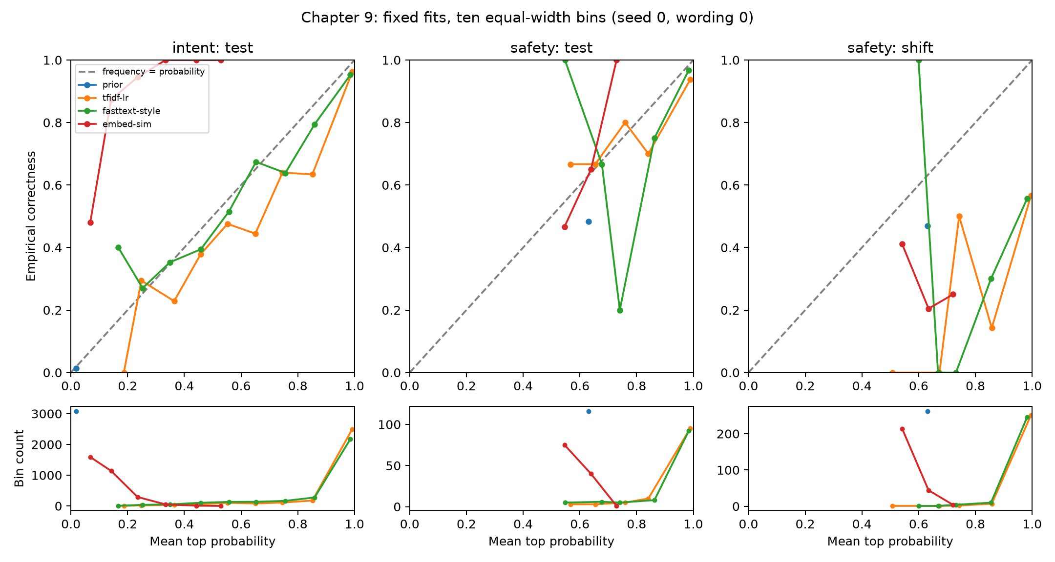
The diagonal asks whether mean top probability matches correctness within a bin. The lower panels show how many observations support each point. An empty region of this diagram supports no claim about requests that land there in production.
OBSERVED, paired intervals at the fixed primary seed/wording:
For intent, LR minus fastText ECE is 0.0111 [-0.0029, 0.0184]; Brier difference is -0.0416 [-0.0551, -0.0279] and accuracy difference 0.0253 [0.0143, 0.0364]. Negative ECE/Brier differences favor LR; positive accuracy differences favor LR. The predicted LR calibration advantage is refuted.
For safety, LR minus fastText ECE is -0.0049 [-0.0397, 0.0382]; Brier difference is 0.0130 [-0.0453, 0.0694] and accuracy difference -0.0086 [-0.0603, 0.0347]. Negative ECE/Brier differences favor LR; positive accuracy differences favor LR. The predicted LR calibration advantage is refuted.
On safety shift, the ECE changes (shift minus test, independently resampled) are tfidf-lr: 0.3782 [0.2877, 0.4411]; fasttext-style: 0.3719 [0.2880, 0.4336]; embed-sim: 0.1287 [0.0175, 0.1966]. These compare different datasets; they do not isolate the cause of the change. The numeric degradation prediction has provider-specific verdicts in metadata.
Across the declared seeds, intent: fastText ECE range 0.0389–0.0423, accuracy 0.8516–0.8526; safety: fastText ECE range 0.0439–0.0675, accuracy 0.8793–0.9052. All seed results and their LR comparisons are retained; the primary table is not seed selection.
Wording variation is intent/test: embedding accuracy 0.5000–0.6799, ECE 0.4209–0.5630; safety/test: embedding accuracy 0.4741–0.6983, ECE 0.0574–0.2205; safety/shift: embedding accuracy 0.3740–0.6641, ECE 0.0399–0.1861. No wording was chosen on test. These ranges do not establish generalization beyond the frozen descriptions.
A probability-shaped number can be useless
OBSERVED: the banking train-prior control has ECE 0.0064 [0.0028, 0.0103], accuracy 0.0130, Brier 0.9878, log loss 4.3820 and AUROC 0.5000, with n=3080. It ranks no state above another. In the exact synthetic class-prior fixture, ECE is 0.0000 while accuracy is 0.6000, AUROC 0.5000, Brier 0.4800 and log loss 0.6730, with n=10. The latter’s finite-sample bootstrap interval is in the results record.
Wrong: the lowest ECE identifies the best decision provider.
Correct: ECE asks one frequency question under one estimator. Read it beside discrimination, proper scoring rules, accuracy and the action’s error costs.
The train-prior control is deliberately boring. It gives every state the same distribution. Its low ECE is not a software defect or proof of useful decisions. It is the case the suite must accept while making its lack of discrimination visible. A provider’s ability to rank requests and its ability to report useful frequencies are distinct requirements.
Bins and sample sizes can move the conclusion
OBSERVED: the preregistered calibrate/threshold search found 3 provider-pair/split cases with a point-estimate ordering reversal. For safety/calibrate, tfidf-lr versus fasttext-style, the ECE differences were width10 0.0070, width15 -0.0070, mass10 -0.0095. The two bin-count/scheme comparisons are reported separately.
| Safety threshold provider | n | Median ECE10 | 95% subsampling spread | Full-sample ECE10 |
|---|---|---|---|---|
| tfidf-lr | 30 | 0.0837 | [0.0226, 0.1584] | 0.0685 |
| tfidf-lr | 60 | 0.0722 | [0.0421, 0.1023] | 0.0685 |
| tfidf-lr | 90 | 0.0685 | [0.0685, 0.0685] | 0.0685 |
| fasttext-style | 30 | 0.1126 | [0.0457, 0.2013] | 0.1051 |
| fasttext-style | 60 | 0.1090 | [0.0732, 0.1502] | 0.1051 |
| fasttext-style | 90 | 0.1051 | [0.1051, 0.1051] | 0.1051 |
| embed-sim | 30 | 0.0954 | [0.0269, 0.2210] | 0.0796 |
| embed-sim | 60 | 0.0756 | [0.0401, 0.1375] | 0.0796 |
| embed-sim | 90 | 0.0796 | [0.0796, 0.0796] | 0.0796 |
The spread comes from repeated subsets without replacement, not an iid confidence interval. Each row also records a declared first-subset example with ECE bootstrap interval, accuracy, Brier, log loss and AUROC. We do not call its median ECE a population error bound.
These comparisons use the declared search space. We did not hunt for a reversal on test or keep changing bins until one appeared. A point-estimate rank flip does not by itself establish a statistically resolved performance reversal. At small sample sizes, bins may describe only a handful of observations. Bootstrap uncertainty is part of the result, and small-n resampling spreads have a different interpretation from confidence intervals.
Normalization is not a calibration method
The existing embedding provider computes cosine similarities and multiplies
them by a positive scalar before softmax. Its parameter is called temperature
in the earlier code, but operationally it is an inverse temperature. Here we
record the multiplier as k. We preserve the earlier operation rather than
silently switching to division.
HYPOTHESIS tested here: changing that positive multiplier keeps the winning label and can change ECE. We did not assume arbitrary scores are miscalibrated by logical necessity. They may happen to be calibrated. What normalization fails to supply is evidence for a frequency interpretation.
OBSERVED, threshold only:
| Task | Multiplier k | ECE10 width [95% bootstrap] | Accuracy | Brier | Log loss | AUROC | n |
|---|---|---|---|---|---|---|---|
| intent | 1 | 0.6506 [0.6196, 0.6805] | 0.6670 | 0.9808 | 4.1304 | undefined | 1000 |
| intent | 10 | 0.5573 [0.5273, 0.5852] | 0.6670 | 0.8339 | 2.5267 | undefined | 1000 |
| intent | 30 | 0.1058 [0.0841, 0.1317] | 0.6670 | 0.4617 | 1.2567 | undefined | 1000 |
| safety | 1 | 0.1478 [0.0483, 0.2377] | 0.6556 | 0.4915 | 0.6846 | 0.7356 | 90 |
| safety | 10 | 0.0796 [0.0350, 0.1717] | 0.6556 | 0.4331 | 0.6243 | 0.7356 | 90 |
| safety | 30 | 0.1182 [0.0641, 0.2225] | 0.6556 | 0.4005 | 0.5806 | 0.7356 | 90 |
Log-loss clipping sensitivity on threshold is retained separately. At the declared epsilon values, intent/tfidf-lr: range 0.0258; intent/fasttext-style: range 0.0212; intent/embed-sim: range 0.0000; safety/tfidf-lr: range 0.0003; safety/fasttext-style: range 0.0429. No threshold, scale or clipping rule was selected from these results.
No scale is selected from this demonstration. Choosing the best one would start Chapter 10’s calibration work and would require its own fitting protocol.
The intent threshold split omits a required class, so its macro AUROC is undefined under the declared rule. The complete intent test split supports the AUROC in the main table. We do not silently drop the missing class.
Jev’s concentration statistic needs its own question
DOCUMENTED — vendor: TypeSafe explicitly distinguishes confidence from
the option probabilities. For a Choice it derives confidence from the selected
probability and answer-set size:
C, untested: the Hacker News discussion contains the claimed confidence errors that motivated this chapter. We cannot confirm them from our absent Jev cache, and a percentage in that discussion is not automatically this chapter’s estimator. Discussion.
3P, not our observation: AnyJev’s historical receipt reports its raw, L0 and L1 readouts on a smaller banking answer set. L1 includes fitted temperature; our chapter fits none. The kickoff warns that its accuracy may reflect teacher agreement. The inspected aggregate receipt does not establish item-label provenance, so we keep that caveat rather than assert independent ground truth. Different answer sets, models and protocols also prevent a direct league table. AnyJev receipt.
The refreshed Red Hat benchmark reports classification comparisons, not a calibration evaluation. Its accuracy findings cannot fill the missing Jev calibration arm.
Put provenance beside the score
PROPOSED: the versioned contract view adds calibration_state without
breaking the earlier constructors. The default is UNCALIBRATED. A CALIBRATED
record requires the dataset or split, sample count, date, method and evidence
reference. The shim upgrades an old result or decision into this view.
The validator checks that the required fields exist and have usable types. It
does not verify that a method worked, that an evidence reference is true, or
that another distribution will behave similarly. Every actual provider in this
chapter remains UNCALIBRATED; measurement alone is not a fitted calibration
method. A provenance field does not make your action safe by declaration.
Run the small demonstration from the repository root:
python examples/ch09-confidence-is-not-probability/demo_ch09.py
The implementation imports the shared harness. Its reference checks, independent hand fixtures and compatibility tests run with:
python -m pytest tests/calibration tests/contract -q
The staged reproduction and evidence verification commands are in the example
README. Stages keep incomplete outputs under results/partial/; the final
results and compressed item distributions appear only after completion.
What you can carry forward
OBSERVED: the predictions have mixed outcomes. ECE bands and shift-degradation thresholds are checked provider by provider, rather than collapsed into a universal claim. The LR-versus-fastText calibration prediction does not authorize selecting the lowest-ECE provider for the application. Binning and sample-size sensitivity are findings under the declared estimators.
PROPOSED conclusion: the contract should carry calibration provenance while keeping its default uncalibrated. A score may support a frequency interpretation on a particular evaluation distribution. These results do not certify that interpretation for an individual request or a future distribution.
The required papers were read partly from full text, with inspected sections recorded. Appendix proofs were not audited. We measured existing providers on fixed public datasets, not general calibration across deployments. Wording bias, finite-sample bias, conditional bootstrap intervals, missing intent shift and the absent hosted/NLI arms bound the conclusion. Untested explanations for a provider’s calibration are hypotheses, not mechanisms established here.
The numeric band prediction held for LR and fastText on both tasks, but failed for embedding in opposite directions: banking ECE was above its predicted band, and safety ECE below it. The predicted LR advantage failed on both tasks; the paired ECE intervals include zero, so these data do not resolve an ECE winner. Shift degradation, the declared binning reversal, scale sensitivity and the small-sample median prediction were observed. The embedding shift interval includes changes smaller than its predicted minimum, even though its point estimate passes that minimum.
Fit wall times are recorded for replay planning. CPU-seconds, peak memory and comparable serving latency were not measured; these results support no cost ranking.
Chapter 10 inherits checked estimators, unfitted calibration splits, fixed per-item outputs, and an explicit place for calibration provenance. What would you have to know before you let a program branch on this number?