What Is Inference?
Distinguish mathematical inference, LLM forward passes, token generation, and production serving, and measure where one request actually spends its time.
I asked a 124-million-parameter model to continue a sentence by sixteen tokens. On a CPU it took about 2.7 seconds. The answer was:
An inference engine takes a trained model and a request, and it must turn them into a model that can be used to generate a model that can be used to generate
Three observations describe this run, but they answer different questions. The request took about 2.7 seconds to produce sixteen new tokens on the recorded CPU configuration. The continuation was repetitive and of little use to a reader. And it was consistent with the requested decoding rule: greedy selection returned the same sequence across the recorded repeat runs. That last observation is evidence of repeatability under these conditions, not proof that every part of the implementation is correct. To establish correctness we must specify the operation, check the implementation against it, and report the scope of the check.
Most of this book is about keeping performance, output quality and implementation correctness separate. Performance asks how long and at what resource cost the computation ran under a declared workload. Quality asks whether the generated text was useful for its task. Correctness asks whether tokenisation, forward computation, token selection and stopping followed their specified rules. One run can be fast but wrong, slow but correct, or correct yet unhelpful. An engineer who confuses these axes may tune the sampler to repair latency, optimise a kernel to repair a prompt, or claim that repeatable output proves an implementation sound. Later chapters will add explicit tests and task metrics instead of treating any one of these observations as a substitute for the others.
This chapter builds the vocabulary and the first measurement. By the end you should be able to say, for one request to one model, which stages ran, which of them were real computation and which were simulated, where the measured time went, and what the measurement does not let you conclude.
Where this sits
This book is one volume in a series that builds a coding-agent system called Pi. The earlier volumes cover the agent loop, language, embeddings, retrieval and memory, and the series plan places optimised language-model programs (DSPy) immediately before this one. Each of them depends on calls to a language model, and in each the cost, delay and behaviour of those calls are a dependency rather than the subject.
This volume opens that box. In the series plan it contributes efficient model execution and provider-level measurements: how a trained model is executed, what that execution costs, and how to measure it honestly. It consumes the calls the earlier volumes make and returns two things: an explanation of what a call does, and an instrument that can tell whether a change to the system made it better. The volumes that follow depend on it: GPU computing takes the kernels apart, model serving puts local models behind provider-compatible interfaces, and evaluation and performance engineering need the measurement discipline built here.
Throughout the book we build the Inference Lab, an inspectable, pluggable runtime for reproducible experiments. It is a teaching and measurement instrument, not a production-engine clone. Each chapter adds a component and records what was implemented, what was simulated and what was actually measured. This chapter adds a request record and stage timings. Designing the Inference Runtime–Implementing Scheduling and Caching–Adding Multiple Model Backends assemble a runtime, scheduler and backend interfaces; Benchmarking Against Established Engines–What We Learned: Inference From First Principles examine comparison methods and the remaining evidence gaps. A comparison with an external engine counts as a result only if both systems actually ran under a matched, recorded workload. Installation checks, unrun plans and provider documentation are not benchmark results.
Four meanings of one word
The word inference is used for four different things, and the confusion between them is the source of most muddled discussion.
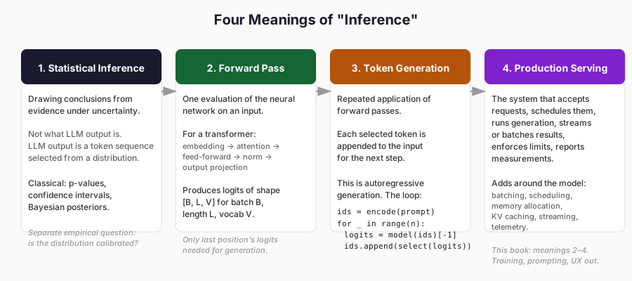
- Statistical inference draws conclusions about unknown quantities from evidence under stated assumptions. A language model also produces conditional probabilities over tokens, but those probabilities do not by themselves establish the truth of a sentence or a calibrated probability that its answer is correct. Calibration requires a specified prediction target and an empirical test. This book concentrates on executing the model and observing its outputs, not treating the model’s token probabilities as statistical conclusions about the world.
- A forward pass is the evaluation of a neural network on an input. For a transformer it applies embedding, attention, feed-forward, normalisation and output-projection operations and produces scores for the next token.
- Token generation is the repeated application of forward passes, with each selected token appended to the input of the next. This is autoregressive generation.
- Production serving is the system that accepts requests, schedules them, runs generation, streams or batches results, enforces limits and reports measurements.
When this book says inference without qualification, it means the path from an already trained model artefact to an observable result: meanings 2–4. We do not train new foundation models or prescribe what a model ought to say. Yet the boundary is porous in engineering terms. A prompt changes token count and cache reuse; a tokeniser revision changes the input; quantisation changes arithmetic; a decoding policy changes the generated sequence. Those interactions belong here because they change the work or its observed outcome. Measuring task success, numerical agreement, policy compliance or quality also belongs here when a performance claim depends on it. Deciding the desired product behaviour is a separate design problem; checking whether a runtime preserves the declared behaviour is an inference problem.
The chain that every chapter preserves
Every chapter in this book is an elaboration of one chain:
model parameters -> request -> tokens -> computation -> generated tokens -> served response -> measured outcome
Each arrow is a transformation that can fail independently, and success at one stage does not imply the next. The table lists, for each stage, what it owns, a failure that is easy to mistake for a failure elsewhere, and where the first chapters of the book let you observe it.
| Stage | Owns | A failure that looks like something else | Observed here by |
|---|---|---|---|
| Model parameters | Learned weights; interpreted alongside architecture, tokeniser and revision | A wrong model artefact can produce plausible but unintended text | Model name recorded here; full manifest added in From Training to Execution |
| Request | Prompt, options, limits | A bad stop condition looks like a slow model | max_new_tokens and stage list |
| Tokens | Text to ids and back | Non-Latin text costs several times more than English | token_counts.py |
| Computation | Tensor operations per step | Redundant recomputation looks like slow hardware | Per-step forward_pass timings |
| Generated tokens | Selection rule, stop rule | Greedy repetition looks like model failure | The repeated output above |
| Served response | Formatting, streaming, transport | Server queueing looks like slow generation | Not yet present: From Inference Loop to API |
| Measured outcome | Latency, throughput, cost, correctness | A single fast run looks like a fast system | --repeat and its summary |
    flowchart LR
    P[parameters] --> R[request]
    R --> T[tokens]
    T --> C[computation]
    C --> G[generated tokens]
    G --> S[served response]
    S --> M[measured outcome]
    G -->|append and repeat| C
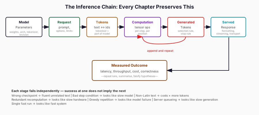
The loop from generated tokens back to computation is the central dependency in ordinary autoregressive decoding: to choose the next token, the model must condition on tokens already chosen. In the baseline used here, generating two hundred tokens therefore entails two hundred sequential model evaluations, with the first evaluation processing the prompt. That does not mean two hundred identical full-prefix computations in an optimised runtime. A key–value cache reuses earlier attention state; batching lets several requests share an iteration; speculative decoding can verify multiple proposed tokens in one target-model pass. The dependency motivates those techniques rather than proving that every engine runs exactly two hundred separate full-sequence passes. Orca’s iteration-level scheduling is an early systems example of treating token-generation iterations as the unit of scheduling.
The autoregressive factorisation
A causal language model defines a conditional distribution over the next token given everything before it:
For a batch of \(B\) sequences of length \(L\), a vocabulary of \(V\) tokens, one forward pass produces logits of shape
First, decode needs the vocabulary scores for the final position, not scores for every earlier position. A straightforward full-sequence language-model call may nevertheless project all positions to vocabulary logits and discard all but the last. For GPT-2, a 768-wide hidden state projected to 50,257 vocabulary entries requires 38,597,376 multiply-accumulates, approximately 77 million FLOPs under the convention of two FLOPs per multiply-accumulate, per position. This is a calculated operation count, not a measured fraction of request latency. Tokens, Embeddings and Probability identifies GPT-2’s tied input/output embedding matrix; Prefill and Decode–Key-Value Caching distinguish prompt prefill, cached decoding and unnecessary repeated work.
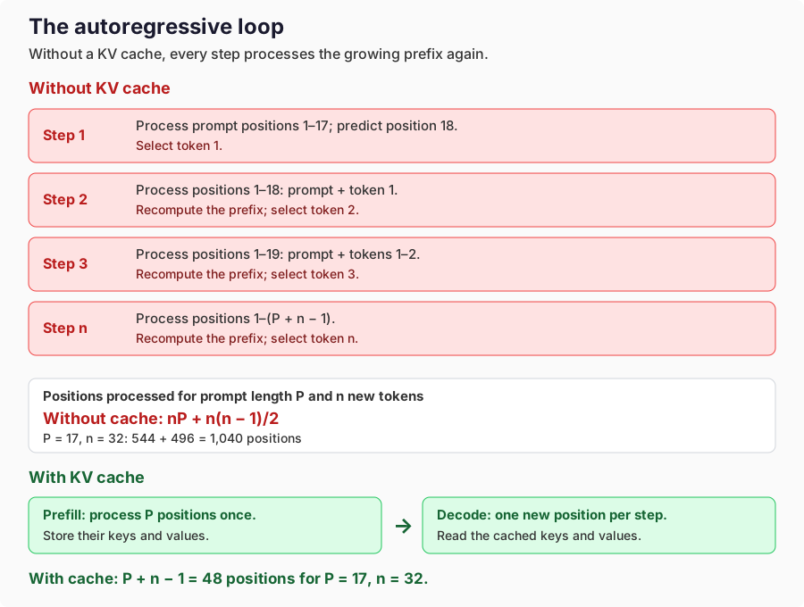
Second, in the deliberately uncached baseline, the input at step \(t+1\) is the preceding input plus the token chosen at step \(t\). Running the complete transformer over that growing sequence recalculates earlier layer states. A KV cache instead stores prior keys and values so decode can process the new position without rebuilding the entire attention history. It does not remove the cost of attending to earlier positions or storing that history. Prefill and Decode measures prefill and decode separately, and Key-Value Caching measures the cache trade-off.
The dependency can be written as short pseudocode. forward_last_position stands for a backend-specific call that returns next-token logits; a real Hugging Face implementation needs tensors, batch dimensions, the model’s output structure and a decision about caching. The runnable Chapter 1 implementation is examples/ch01/inference_stages.py:
ids = encode(prompt)
for _ in range(max_new_tokens):
        logits = forward_last_position(ids)  # abstract model call; not executable as written
    next_id = select(logits)         # greedy, sampled, constrained...
    ids.append(next_id)
    if stop(next_id, ids):
        break
return decode(ids)
Everything else in this book is either making model(ids) cheaper, making the loop less wasteful, deciding which requests share the machine while it runs, or measuring whether any of that worked.
The Inference Lab, stage by stage
The first implementation deliberately contains no neural network. It exposes the stages a real system has so that each can be timed and, later, replaced. The stages are:
request_parsevalidates and normalises the request.tokenizesplits text into model-facing symbols.encodemaps symbols to integer ids.forward_passcomputes scores for the next token.sampleselects a token.decodemaps ids back to text.response_formatassembles the response.
A production system adds scheduling, batching, cache management, memory allocation, streaming and telemetry. These seven stages describe the toy path: it times request_parse, tokenize, encode, per-token forward_pass and sample, decode, and response_format. The real-model path uses the same GenerationResult protocol but combines tokenisation and encoding into tokenize_and_encode, times per-token forward_pass and sample, and times decode. It does not report request_parse or response_format as separate measurements. A common result type does not imply identical instrumentation, so stage-by-stage comparisons must first align definitions.
Each request produces a GenerationResult, defined in examples/ch01/inference_stages.py:
@dataclass
class GenerationResult:
    prompt: str
    tokens: List[str]
    token_ids: List[int]
    text: str
    timings: List[StageTiming]
    simulated_stages: List[str]
    metadata: dict
Two fields matter more than they first appear. timings is an ordered list of (stage, seconds) pairs, so a per-token stage appears once per generated token and the order of events is preserved. simulated_stages is a list of the stages that did not do real work. A result that cannot say which of its stages were simulated cannot safely be compared with one that can.
The ToyGenerator implements the interface with a seeded table. Its forward pass looks up a row of scores for the previous token and applies a numerically stable softmax:
logits = self._logits(previous_id)
maximum = max(logits)
exps = [math.exp(value - maximum) for value in logits]
total = sum(exps)
probs = [value / total for value in exps]
Subtracting the maximum before exponentiating changes nothing mathematically and prevents overflow, a pattern that recurs in attention. Selection is greedy with a deterministic tie-break on the smallest token id, so a fixed prompt, seed and length always give the same result.
Run it from the repository root:
python examples/ch01/inference_stages.py "Hello" --max-new-tokens 8
python examples/ch01/inference_stages.py "Hello" --max-new-tokens 8 --json
For seed 7 the eight generated characters are RWPFdyxf. That output is meaningless as language, and that is the point. The toy is a test fixture for the interface and the timing harness. It is not evidence about model quality, hardware or serving.
What is simulated
The toy result’s simulated_stages field contains three labels. They do not all describe the same kind of substitution:
forward_passis a surrogate computation: a table lookup, bias addition and softmax over 57 characters, not learned transformer layers or attention.sampling_distributionlabels a surrogate distribution. The program really performs greedy selection in the timedsamplestage, but it selects from artificial scores rather than a trained language-model distribution.kv_cachelabels an absent capability. The toy only examines the preceding character and has no attention history to cache. No cache is executed or timed.
The record is explicit, but a future version of the schema should distinguish SIMULATED from NOT_IMPLEMENTED rather than combine them in one list. Here the list is a warning about interpretability, not a measurement of those capabilities. Building Our First Inference Engine will adapt the common interface to a real model backend; it must not turn these missing capabilities into apparent measurements.
The real model
The same interface drives a real model. RealModelRunner wraps a Hugging Face causal language model, loads it once, and records the same stage timings. It decodes greedily and, deliberately, has no cache: every step runs the model over the whole sequence so far. That is the baseline that later chapters improve on, and it should be measured before it is improved.
Experiment design
The question is narrow: for a small model on a CPU with no optimisation, where does the time of one request go?
- Hypothesis (book hypothesis before measurement). For this model, prompt and single-thread CPU configuration, the forward pass will dominate the timed in-process stages. Without a cache, later steps will process more positions and should tend to take longer, after warm-up and run-to-run noise are accounted for.
- Held constant. Model
gpt2(124,439,808 parameters), snapshot607a30d783dfa663caf39e06633721c8d4cfcd7e, greedy decoding, one prompt of 17 tokens, 16 new tokens, CPU, PyTorch 2.6.0+cu124, Transformers 5.17.0, one PyTorch intra-op thread, offline model cache, Windows 11, a single machine. - Varied. Number of requests: one process with one request, and one process with five consecutive requests against a loaded model. Within each request, the prefix grows by one token per step.
- What would count against it. A substantial non-forward share would contradict the first prediction. An adequately replicated study varying prompt length independently of generation step could contradict the predicted positive length–latency trend. A flat line in one noisy run would not establish that the program stopped recomputing the prefix; that is visible from the code, while the runtime cost is what this measurement probes.
python examples/ch01/inference_stages.py "An inference engine takes a trained model and a request, and it must turn them into" --max-new-tokens 16 --real --json
python examples/ch01/inference_stages.py "An inference engine takes a trained model and a request, and it must turn them into" --max-new-tokens 16 --real --repeat 5 --json
Both runs used the model from a local cache. They download nothing and call no paid service. Results are recorded in research/ch01/results.json.
Where the time went
Over five requests (80 forward passes) against one loaded model:
| Stage | Count | Median | Min | Max | Total |
|---|---|---|---|---|---|
forward_pass |
80 | 177.9 ms | 124.2 ms | 249.8 ms | 13.93 s |
sample |
80 | 0.40 ms | 0.37 ms | 1.23 ms | 0.034 s |
tokenize_and_encode |
5 | 0.30 ms | 0.25 ms | 2.94 ms | 0.004 s |
decode |
5 | 0.14 ms | 0.14 ms | 0.27 ms | 0.001 s |
Across these five requests, the 13.93 seconds assigned to forward_pass are about 99.7% of the summed, instrumented stage durations. That is not a share of process startup, model loading, transport, queueing or end-to-end service latency: none of those costs appears in the table. The observation is unsurprising for a 124-million-parameter model with a 50,257-token vocabulary running full-prefix forwards on a single CPU thread. The informative quantity is the measured gap between stages: median selection took about 0.40 ms per token against 177.9 ms for the forward pass. It would be a mistake to generalise that split to GPU kernels, a batched service or a different decoding policy.
Model loading is not in that table, because it happens once per process. It took 3.20 s in the single-request run, 1.58 s in the repeat run, and 2.37 s in the run recorded when this example was first written. Those three numbers come from three processes on one machine. A factor of two between them is a warning that load time depends on file caching and operating-system state, and that a single load measurement is a weak basis for any claim.
The five requests produced identical text, and their durations were 2.70, 2.67, 2.86, 2.82 and 2.92 seconds. The request-level totals do not show a consistent first-request slowdown after model loading. In a different single-request process, however, the first forward pass took 0.403 s and the next 0.132 s. Those observations are compatible: an isolated first-pass penalty can be obscured by the sum of sixteen steps and ordinary variability. Neither run isolates its cause. From Training to Execution uses fresh processes to examine import time, model loading and first-forward warm-up separately; this chapter makes no causal claim from the first-step observation.
Per-step cost without a cache
The single-request run recorded each forward pass in order. The 16 values, in milliseconds, were:
403.1  132.2  136.8  149.8  157.1  151.3  153.8  164.6
171.4  179.8  179.9  183.4  173.6  188.5  207.6  209.0
Excluding the first forward pass, the recorded time grows from 132 ms at 18 processed positions to 209 ms at 32, about 1.6 times as long for about 1.8 times as many positions. This is consistent with full-prefix recomputation, which the uncached code performs, but is not a controlled estimate of the cost of adding a token. Position count and decode-step index move together, and these sixteen observations come from one run with no independent replication. To test the scaling claim rather than merely illustrate it, vary prompt length independently of step index, repeat the runs, report dispersion and check for warm-up effects. The fourth exercise below starts that experiment; Prefill and Decode and Key-Value Caching develop the mechanism.
A rough model gives the right scale without pretending to profile the hardware. Multiplying roughly 124 million parameters by two FLOPs per parameter per token yields about 0.25 GFLOP per position for dense parameter operations. At 18 positions that is around 4.5 GFLOPs; divided by 0.132 s it implies roughly 34 GFLOP/s in this simplified accounting. This omits or approximates attention’s sequence-length-dependent operations, reused/tied parameter effects, numerical kernels and non-arithmetic overhead. The timing is measured, but the operation count and inferred throughput are estimates, not observed hardware throughput. Memory Bandwidth and Compute Bottlenecks will examine the compute/bandwidth distinction on an appropriately instrumented workload.
The output is a separate question
The generated continuation repeats itself. Greedy selection takes the highest-scoring next token at every step; that rule can reinforce a local pattern as the selected text becomes the next input. Holtzman et al., in The Curious Case of Neural Text Degeneration, document repetition and other failure modes of likelihood-maximising decoding and study alternative sampling strategies. Their result provides research context, not independent validation of this particular GPT-2 run. The recorded observation here is narrower: with this artefact, prompt and greedy rule, the implementation returned the same repetitive sequence in five requests. That observation alone does not prove every kernel correct or identify a single cause of the output’s poor usefulness.
This is the chapter’s clearest example of why faults should be assigned to the right layer. The observation is not that GPT-2 is intrinsically incapable of coherent text, or that faster execution would fix this continuation. It is that greedy decoding of this checkpoint on this prompt repeats. Changing the decoding rule can change the continuation while leaving the underlying model weights and core forward computation unchanged. Changing the execution engine may change latency, memory use and numerical behaviour; it is not guaranteed to preserve every token unless numerical agreement and decoding parity have been checked. Tokens, Embeddings and Probability, Correctness, Determinism and Reproducibility and Adding Multiple Model Backends put tests around those distinctions.
Toy and real side by side
The toy forward pass had a median of 5.7 microseconds over 80 steps. The real one had a median of 177.9 ms. That is a ratio of roughly 31,000, and it must not be read as an optimisation figure in either direction. The toy does a table lookup. The real model does matrix multiplications with 124 million parameters. The comparison is there to make the boundary visible: the toy exercises the interface and the timing harness, the real model exercises the computation, and only the second is evidence about transformer inference.
Tokens are the unit of work
The toy generator treats each character as a token. Real models do not. A tokeniser maps text to a sequence of integer ids drawn from a fixed vocabulary, and everything that is counted later, including context limits, per-token prices, cache size and throughput, is counted in those tokens rather than in characters or words.
examples/ch01/token_counts.py compares characters, UTF-8 bytes and GPT-2 tokens for four short samples:
| Sample | Characters | UTF-8 bytes | Tokens | Characters per token |
|---|---|---|---|---|
| English sentence | 56 | 56 | 11 | 5.09 |
| Python code | 57 | 57 | 23 | 2.48 |
| Digit string | 31 | 31 | 12 | 2.58 |
| Japanese sentence | 26 | 78 | 37 | 0.70 |
These four different, hand-picked strings require between 11 and 37 GPT-2 tokens. The Japanese example has fewer characters than the English sentence but more than three times as many tokens; the code and digit examples have their own segmentation patterns. Because the strings do not convey identical content, the table is not a controlled comparison of languages or tasks. It demonstrates why character count is not a portable proxy for token count. The inference engine must record which tokeniser version produced the ids, because context length, billing and cache behaviour are defined over those ids. Tokens, Embeddings and Probability tests tokenisation and token selection in more detail.
What the numbers do not show
The measurements above are narrow, and it is worth being explicit about how.
- One machine, one session. Nothing here is a portable performance result. The environment is recorded so the experiment can be repeated, not so the numbers can be compared with anyone else’s.
- One thread. PyTorch was using one intra-op thread. A configuration using the machine’s 24 logical CPUs would give different absolute times and perhaps a different split.
- One prompt and one model. The per-step trend might look different at 1,000 tokens, and a larger model would shift the balance between forward pass and everything else.
- Wall-clock timing with Python overhead. The
timingslist measures elapsed time around each stage, including interpreter and library overhead. It does not separate arithmetic from memory movement. Memory Bandwidth and Compute Bottlenecks does that. - No GPU, no batching, no concurrency, no memory measurement. These are not measured. They are recorded as not measured in the results file, not omitted from it.
- Model identity was recorded by hand. The program stores the model name
gpt2but not the snapshot revision. The revision above was read from the cache directory afterwards. Provenance that depends on a human remembering to write it down will eventually be wrong. Closing that gap is the first exercise on the Inference Lab.
Inference Lab increment
This chapter adds the request record: a GenerationResult carrying output, ordered stage timings, the list of simulated stages and metadata. Its interface is the TokenGenerator protocol:
class TokenGenerator(Protocol):
    def generate(self, prompt: str, max_new_tokens: int) -> GenerationResult: ...
Anything that satisfies the protocol can be timed by the same harness, repeated by run_repeated, and summarised by summarise_timings. The toy and the real model already satisfy it, which is the first small demonstration that an engine can be swapped under a fixed interface and measured the same way. The multi-backend chapter, number 43, generalises this idea, and the benchmark chapters rely on it.
Two limits of the record are already visible and are intentionally left in place. It has no notion of concurrent requests, so it cannot yet express queueing delay. And its metadata is a free-form dictionary, so nothing enforces that two results are comparable. Both are addressed in the service and benchmarking parts of the book.
What you should now be able to do
- Say which of the four meanings of inference a given statement is about, and name the meaning that this book uses.
- Explain why ordinary autoregressive decoding has one dependent token-selection iteration per output token, and how KV caching, batching and speculative verification change the work performed in those iterations.
- Run one request against a real model, read the stage timings, and say which stage dominates and by what margin.
- Distinguish a slow result, a poor result and a correct result, and say which part of the chain each belongs to.
- State at least three things a given measurement does not allow you to conclude.
Key terms
- Inference: executing a trained model on an input to produce an output.
- Forward pass: one evaluation of the model’s layers on a given input.
- Autoregressive generation: producing tokens one at a time, feeding each output back as input.
- Logits: unnormalised scores over the vocabulary before selection.
- Token: the discrete unit a model reads and writes, defined by a specific tokeniser.
- Greedy decoding: selecting the highest-scoring token at every step.
- Sampling: selecting a token randomly according to a distribution derived from the logits.
- Stage: a named step in the request path whose duration is recorded separately.
- Serving: the system that manages requests, execution and responses around the model.
- Simulated stage: a stage that returns plausible output without performing the real computation.
Reader exercises
- Modify
ToyGeneratorto sample from the softmax distribution using a fixed seed instead of greedy selection. Which stages change? Which stay identical? Does repeatability survive? - Add a stop reason to
GenerationResult(length reached, end-of-sequence, stop string). Decide whether the stop reason belongs to generation or to serving, and defend the choice. - Extend
RealModelRunnerto record the snapshot revision and tokeniser name inmetadataautomatically, and add a test that fails if either is missing. Why is a free-form dictionary a risky place for this? - Run the repeat experiment with prompts of 8, 64 and 256 tokens and the same 16 new tokens. Plot median forward time against position processed. Does the shape support the hypothesis that each step pays for the whole prefix? What would it have to look like to falsify it?
- Set
torch.set_num_threadsto 1, 4 and 12 and repeat the experiment. Does the forward-pass share of request time change? Does the step-time trend? - Write one claim from this chapter that your experiments could falsify, and the measurement that would do it.
References
- Transformer computation — primary research: Vaswani et al. (2017), Attention Is All You Need. Establishes transformer attention and decoder-side masking; it does not measure the local GPT-2 run.
- Decoding and repetition — primary research: Holtzman et al. (2019), The Curious Case of Neural Text Degeneration. Provides evidence about degeneration under maximising decoding objectives and motivation for nucleus sampling; it does not show that sampling always improves task correctness.
- Scheduling and serving — primary research: Yu et al. (2022), Orca: A Distributed Serving System for Transformer-Based Generative Models. Introduces iteration-level scheduling and selective batching; its reported system performance is not reproduced by this chapter.
- Implementation documentation: Hugging Face Transformers generation strategies documents selection, stops and cache configuration; PyTorch 2.6 documentation documents the tensor and thread interfaces used in the local experiment.
- System reference, not a local benchmark: deepseek-ai/DeepInfer at 774ce244 provides first-party code and documentation for a broader inference stack. Its public repository does not by itself establish hosted-service performance or reproduce a result here.
Evidence in this chapter
| Claim | Category and limit |
|---|---|
| Causal attention can compute next-token conditionals from a prefix | Established background; Vaswani et al. (2017) for transformer masking, plus probability chain rule |
| Ordinary autoregressive generation has sequential token dependencies | Established background; not a claim that every engine recomputes each prefix |
| Greedy decoding can produce repetitive continuations | Research context: Holtzman et al. (2019); chapter shows one GPT-2 trajectory |
| Iteration-level scheduling addresses multi-iteration generation workloads | Research context: Yu et al. (2022); not benchmarked here |
| Prefix length contributes to uncached decode cost | Book hypothesis about measured latency; one weakly supportive single-run trend |
| Approximately 0.25 GFLOP per position for GPT-2 under a 2-FLOP-per-parameter heuristic | Arithmetic estimate, not a profiler measurement |
forward_pass was about 99.7% of the instrumented in-process stages in this configuration |
Book result from five requests in research/ch01/results.json; excludes loading and service overhead |
| Token counts of four hand-picked samples under the GPT-2 tokeniser | Book result in research/ch01/results.json; not a language comparison |
| GPU execution, service queuing, memory, batching and real multi-request throughput | Not measured in this chapter |
| Output quality, semantic correctness and model calibration | Not evaluated in this chapter |