Prefill and Decode
A request does two different jobs. Measured on a real model: what each costs, where the textbook bottleneck fails for a small model, and how a long prompt stalls everyone else.
On the measured RTX 2060 workstation, one cached GPT-2 request took about 12 ms to produce its first token from a 16-token prompt, followed by roughly 11 ms per subsequent token. For a 1,000-token prompt, the measured first-token interval rose to about 44 ms, while later-token intervals remained near 11 ms. The phase shares reverse when the requested reply changes length: the 16-token prompt followed by 64 output tokens spent about 98% of measured model-loop time after the first token; the 1,000-token prompt followed by four output tokens spent about 56% before the first. Those are local measurements of a cached, greedy GPT-2 loop, not client-visible service latencies.
One request contains two different workloads. Prefill processes a known prompt in parallel and builds attention state; decode conditions each successive choice on earlier choices, reusing that state. Their costs respond differently to prompt length, output length, kernel overhead, weight traffic and scheduling. In a separate two-request simulation, inserting a 1,000-token prefill during another request’s stream increased its largest inter-token gap to 56–73 ms, against a typical gap of roughly 11–13 ms. This is an interference observation under one sequential schedule, not a measurement of a production server.
The familiar rule is that prefill tends to be compute-intensive and single-token decode tends to be bandwidth-sensitive. That rule is a workload-dependent performance model, not a property guaranteed by transformer mathematics. This chapter tests the rule with GPT-2 small on a Windows workstation. The short-prompt and per-token measurements are consistent with a substantial fixed execution overhead; they do not isolate CPU dispatch, CUDA launches, cache maintenance or host synchronisation well enough to prove which one is the bottleneck. We will retain the measured numbers and keep the proposed causes separate from them.
Where this sits
Autoregressive Generation distinguished parallel scoring from serial token selection. Matrix Multiplication and GPU Execution introduced arithmetic intensity, the roofline bound and host-side execution overhead; Attention and Its Computational Cost distinguished prefill-shaped \(T\times T\) attention from decode-shaped \(1\times T\) attention against stored keys and values. Here these pieces form the two phases of a request. Chapter 9 measures phase latency; Key-Value Caching will measure the consequences of using and not using a KV cache under controlled comparisons.
The Inference Lab increment is a small measurement vocabulary: request_metrics turns a timestamp trace into TTFT, ITLs, TPOT and end-to-end time; phase_share divides two measured phase durations; chunk_schedule partitions prompt positions. There is also a helper named goodput, but it currently returns an SLO-compliance fraction, not goodput in requests per second. The difference matters whenever rates, admission policy or system capacity are compared. These pure helpers have CPU-runnable tests; the GPU results below are separately recorded experiments.
The experiments use the library’s KV cache as a black box. The phases can be defined without a cache, but keeping previous keys and values is what makes a one-position incremental decode step possible without recomputing the entire prefix. The cached-versus-uncached performance comparison is not carried out here. Key-Value Caching implements caching more explicitly, checks numerical agreement and measures the work it avoids.
For the Pi series, agent traffic illustrates why these phase measurements matter. A tool response or retrieved passage may produce a long input and a short completion; an assistant writing a long answer to a short query is the opposite shape. These are workload examples, not fixed classifications: repeated history, cache reuse, batch size, output length and queueing can all change which phase dominates. The practical question is what proportion of the actual request budget goes to each phase under the intended workload.
Two phases

Prefill evaluates a prompt containing \(T\) known tokens. At each layer the model projects all prompt positions and, when caching is enabled, retains their keys and values. The final prompt position’s logits give the probability distribution from which the first generated token can be selected; a further one-token forward pass is not required to obtain it. Our examples request only the last logits row (logits_to_keep=1) and record the resulting model-call time. They do not include tokenisation or client transport.
Decode begins after that first token has been selected. The next forward pass consumes that token at its new position, reads the previously cached keys and values for each attention layer, extends the cache and produces logits for the second generated token. Repeating this yields a serial chain of selections, although the matrix work inside each step is parallel. Thus, for \(n\) generated tokens in the cached experiment, there is one prefill and \(n-1\) subsequent decode forward passes; an implementation that counts \(n\) of each has an off-by-one error.
At the attention level, a full causal prefill concerns \(T\) query positions and up to \(T\) visible key positions, while a cached decode step has one new query and approximately \(T\) cached keys. For the weight projections the corresponding row counts are \(T\) and one. These shapes explain the different scaling opportunities, but shape alone cannot establish whether a measured implementation is launch-, bandwidth- or compute-limited. It also matters whether prefill computes logits for every prompt position or only the last one.
Use five separate concepts rather than one ambiguous number called “latency”. The first four can be computed for individual token-delivery traces; the fifth additionally requires a population of requests and a time window:
- Time to first token (TTFT): client request submission to receipt of the first output token. In this chapter’s model-only tests the start and end are local timestamps, so the reported value is not client TTFT.
- Inter-token latency (ITL): each elapsed interval between successive delivered output tokens. A trace of \(n\) tokens has \(n-1\) such gaps.
- Time per output token (TPOT): here, the mean of those gaps, \((t_{\mathrm{last}}-t_{\mathrm{first}})/(n-1)\) for \(n\ge2\). For one output token TPOT is undefined; the teaching helper currently returns
0.0instead, which must not be interpreted as a successful decode-latency measurement. - End-to-end latency (E2E): request submission to completion/last delivery; distinguish that from time inside the model loop.
- SLO compliance and goodput: compliance is the fraction of completed requests satisfying configured latency bounds; goodput is the rate of compliant requests, normally requests/second over a defined interval. The current
goodput()helper implements the former, despite its name.
TPOT is a mean; ITL is a distribution. Two streams may have the same TPOT but sharply different longest gaps. The unit tests demonstrate this with constructed timestamps. Accordingly, a benchmark should publish TTFT, mean TPOT, and the ITL tail (for example p95, p99 or maximum with the sample count), alongside request and token rates. With only a handful of tokens, a maximum is a useful observation but not a reliable population tail estimate. Do not derive client-side metrics from GPU events, because queueing, decoding, transport and back-pressure also matter.
The original examples/ch09/prefill_decode.py illustrates two common mistakes. It added a purported first decode step to prefill when calculating TTFT, even though prefill already produced first-token logits; and its “decode” re-ran the whole growing prefix without reusing the cache. The measured implementation, examples/ch09/phases.py, does use past_key_values for incremental work and selects the first token from prefill. Both files still exist: the original example remains a historical fixture, not a correct timing reference for cached decode.
Prefill

The prefill command measures the model call for \(T\) synthetic token ids, with caching enabled and logits restricted to the last position. It records medians from two separate runs of the command, each with its own within-run repetitions (15 timed samples per GPU case, four per CPU case after warm-up). The call operates on ids already resident on the selected device and synchronises for CUDA timing. It does not measure prompt tokenisation, disk/model loading, network time or queueing.
| Prompt tokens | GPU fp32 | GPU fp16 | CPU, 1 thread |
|---|---|---|---|
| 1 | 11.5 – 12.2 ms | 11.9 – 12.0 ms | 40 – 45 ms |
| 16 | 11.6 – 12.5 ms | 13.6 – 14.0 ms | 86 – 95 ms |
| 128 | 11.8 – 12.5 ms | 11.8 – 12.9 ms | – |
| 256 | 12.2 – 15.4 ms | 12.4 ms | 1,037 – 1,070 ms |
| 512 | 22.6 – 26.3 ms | 12.1 – 12.5 ms | 2,096 – 2,111 ms |
| 1,024 | 45.1 – 52.0 ms | 16.1 – 18.3 ms | – |
The timings suggest three useful regimes, but the boundary between them is not identified by direct profiler evidence.
A substantial fixed-time region. GPU fp32 prefill is roughly 12 ms from one to 128 tokens and remains between 12.2 and 15.4 ms at 256; fp16 stays near 12–14 ms through 512 tokens in the two recorded runs. The flatness is consistent with fixed per-operation and host-side overhead (Matrix Multiplication and GPU Execution), potentially including cache and framework bookkeeping. This experiment did not independently time Python dispatch, individual kernel launches, host synchronisation and device computation, so calling the entire interval “launch-bound” is a diagnostic hypothesis, not a verified component attribution. At longer prompts the compute term becomes more visible.
A growing-work region. At 1,024 tokens, the fp32 run measured 45.1–52.0 ms, or approximately 19,700–22,700 prompt tokens/s, with 3.7–4.3 nominal matmul TFLOP/s under the chapter’s operation-count convention. The fp16 run measured 16.1–18.3 ms, or about 56,100–63,800 tokens/s, with 10.6–12.0 nominal TFLOP/s. These figures show much greater effective parallel work than at short prompts. They do not, by themselves, establish that compute throughput is the limiting resource. The operation count is a cost-model estimate (and assumes ideal causal attention where relevant), while the wall-clock interval also includes elementwise work, cache construction and framework overhead.
One CPU thread. In the recorded 64-, 256- and 512-token fp32 prefill cases the CPU sustained about 239–253 prompt tokens/s. This is evidence about the selected one-thread CPU configuration, not about all CPUs. The CPU has its own invocation, memory and scheduling overheads; it simply does not pay the same CUDA submission path. At four prompt tokens the two runs took 71–86 ms, illustrating how rapidly short-sequence throughput changes with workload shape.
Computing less of the output
The Transformer as a Computation predicted that generating only the final logits row can remove roughly 30% of nominal matrix arithmetic for a sufficiently long short-context prefill. Here logits_to_keep=1 makes that operation explicit. At 64, 256 and 512 tokens, the two CPU runs show measured savings of approximately 25–31%, broadly consistent with the arithmetic estimate. At 512 and 1,024 tokens the fp32 GPU savings were about 20–21%. For very short GPU prompts the results are noisy and occasionally negative, so the prediction should not be described as confirmed at every length. The measurement establishes that trimming unused logits can help; identifying why the observed percentage differs from the FLOP percentage requires a more detailed performance breakdown. Importantly, logits_to_keep=1 changes the output projection’s shape and can change floating-point rounding, so numerical equivalence still needs to be checked.
Decode
For each decode configuration, the experiment first builds a library cache from a synthetic prompt of 16, 128, 512 or 960 tokens. It then executes 40 greedy GPU decode steps (12 on CPU), reads each chosen id back with .item() and reports the median after dropping the first four steps. This is a host-synchronising Python loop, not an event-only kernel benchmark. The 960-token case stays within GPT-2’s learned 1,024-position limit; an earlier attempt at 1,000 prompt tokens plus 40 decode steps exceeded that limit and was discarded. The table shows the ranges across two runs.
| Context at start | GPU fp32 | GPU fp16 | CPU, 1 thread |
|---|---|---|---|
| 16 | 11.1 – 11.2 ms | 11.0 – 12.2 ms | 35 – 43 ms |
| 128 | 11.1 – 11.7 ms | 11.3 – 11.6 ms | 39 – 42 ms |
| 512 | 10.9 – 11.4 ms | 11.1 – 11.4 ms | 41 – 76 ms |
| 960 | 10.9 – 11.4 ms | 10.8 – 11.1 ms | – |
Within the measured GPU contexts, the per-step medians remained near 11 ms for both fp32 and fp16, with no sustained increase from starting context 16 to 960. This does not mean decode time is mathematically independent of context: causal attention still reads more cached positions, and the reported 40-step runs move through progressively longer contexts. It means that any change due to those extra positions was not resolved above the roughly 11 ms end-to-end local loop-step cost on this hardware and software stack. The precision comparison is likewise limited to the tested implementation, shapes and two runs.
A bandwidth-only back-of-the-envelope bound gives a useful scale, not a diagnosis. The fp32 model has about 474.7 MiB of parameter storage; the idealised parameter-plus-cache byte count spans roughly 476–542 MiB across the tested starting contexts. Dividing by the 303 GB/s bandwidth reference from Matrix Multiplication and GPU Execution yields about 1.6–1.9 ms if those bytes must traverse that interface exactly once at the reference rate. Yet the measured full Python step is near 11 ms. The ratio of nominal bytes to step time is 43–52 GB/s in fp32 and roughly 20–26 GB/s in fp16. Neither ratio is measured memory-controller bandwidth nor hardware utilisation: parameter or KV reads can be cached, memory traffic may be higher or lower, and other phases contribute time. The disagreement makes a pure, ideal-bandwidth explanation insufficient; it does not identify the real bottleneck.
The most plausible explanation is a significant fixed cost from a sequence of framework calls, GPU launches, cache management and a forced host readback on every token. The experiment does not apportion the observed ~11 ms among these causes, and it cannot infer that no useful cache benefit exists: it never compares cached and uncached generation at matched contexts. Matrix Multiplication and GPU Execution’s single-token forward-pass numbers came from another harness with different input and output conditions, so they are suggestive rather than a controlled subtraction. The next experiment to run is a four-way ablation of cached/uncached execution and synchronous/deferred host token readback, with CUDA event timing and a profiler trace.
The CPU results are more variable: 35–43 ms at a 16-token starting context, 39–42 ms at 128, and 41–76 ms at 512 in the two recorded runs. Those measurements neither isolate memory bandwidth nor establish a reliable context-length slope, particularly at 512 tokens. They do show that a one-thread CPU and this GPU have different performance envelopes for the same algorithm. A clean CPU benchmark would need more repetitions, process isolation and a profile of the relevant matrix and cache operations.
What would make decode bandwidth-bound
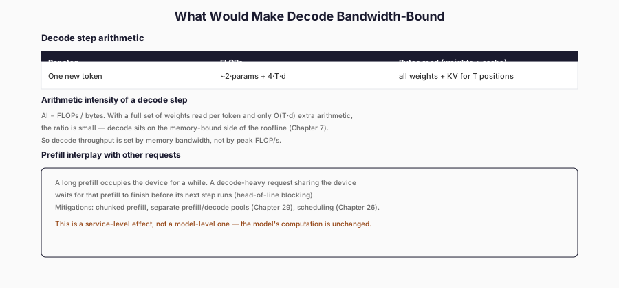
The balance can change radically with model size. For a hypothetical 7-billion-parameter model in fp16, its weights alone occupy approximately 14 GB decimal before any KV cache or temporary storage. Streaming 14 GB once across a 303 GB/s memory interface would take at least 46 ms under an idealised one-read assumption. That is a thought experiment, not a benchmark: this model would not fit within the workstation’s 12 GiB card, real kernels may reuse data or move more bytes, and larger architectures also change launch counts, cache traffic and parallelism. The example explains why weights can dominate at scale; it does not establish the exact transition point or promise a 46 ms decode time.
The practical rule is measure before applying an optimisation. Compare the measured step to arithmetic and data-movement lower bounds, but do not mistake the difference for proof of a specific bottleneck. For a proposed weight quantisation, measure wall-clock latency, GPU execution, memory traffic and output agreement; for launch optimisations, compare a synchronised Python loop with CUDA events and captured/compiled execution. The same model can move between regimes as batch size, context and implementation change.
Where the time goes in a request
The next table comes from cmd_endtoend: five runs per case, cached greedy decode, last-position prefill logits, synthetic prompts and fp32 GPT-2 on the GPU. First-token time is measured from the start of the local prefill call to the first token’s host readback; subsequent ITLs come from timed cached decode steps. The request_metrics helper uses a reconstructed timestamp trace for those decode steps. The phase shares are computed from separately aggregated median prefill and decode durations, so small differences from the end-to-end median are expected.
| Prompt | Output | TTFT | TPOT | End to end | Prefill share | Decode share |
|---|---|---|---|---|---|---|
| 16 | 64 | 12.3 ms | 11.2 ms | 720 ms | 1.7% | 98.3% |
| 128 | 64 | 11.8 ms | 11.4 ms | 731 ms | 1.6% | 98.4% |
| 512 | 64 | 23.1 ms | 11.5 ms | 747 ms | 3.1% | 96.9% |
| 512 | 8 | 22.8 ms | 11.4 ms | 102 ms | 22.1% | 77.9% |
| 1,000 | 16 | 43.6 ms | 11.1 ms | 211 ms | 20.6% | 79.4% |
| 1,000 | 4 | 43.9 ms | 11.3 ms | 78 ms | 56.3% | 43.7% |
In these six configurations measured local TTFT rises with prompt work once the prompt leaves the nearly flat short-input region, while TPOT remains near 11–11.5 ms. The share assigned to prefill ranges from about 1.6% (128 prompt, 64 output) to 56.3% (1,000 prompt, four output). These are not universal relationships: batch size, longer context, sampling, output post-processing and queueing can shift both phases. For an actual retrieval or agent workload, record its real prompt/output length distribution before deciding which phase deserves optimisation.
The label TTFT needs an explicit timing boundary. cmd_endtoend starts its clock immediately before the model’s prefill call, uses already-created GPU token ids, and ends the first-token interval after argmax and .item() have synchronised the selected token to the host. This local model-loop TTFT excludes tokenisation, scheduling/queueing, input transfer from the client, network delivery and client rendering. Its “end-to-end” column is likewise end-to-end within this model-loop scope, not service end-to-end latency. The trace is reconstructed from the recorded per-step durations rather than directly timestamping an HTTP stream. From Inference Loop to API can introduce external request and client-delivery boundaries; until then the tables should retain the narrower labels.
When one request’s prefill hurts another
To expose one scheduling trade-off, the harness simulates two requests in a single Python process on one GPU, with model calls executed serially. Request A decodes after a 32-token prompt. At A’s tenth decode step, request B enters with a 1,000-token prompt. B is processed either in one prefill call or in cache-preserving chunks, with one B chunk interleaved after each A decode step. The experiment records A’s token gaps and the time until B’s last prefill chunk has completed and its final logits are available. It does not simulate a queue of independent arrival processes or client/network token delivery.
Across three command runs, the following ranges were observed. The last column is labelled B prefill-completion interval, not service TTFT: the harness synchronises B’s final logits but does not sample, emit or transport B’s first token.
| B’s prefill chunk (tokens) | Worst local gap in A | Median local gap in A | B prefill-completion interval |
|---|---|---|---|
| 1,000 (unchunked) | 56–73 ms | 11–13 ms | 56–76 ms |
| 512 | 39–51 ms | 11–13 ms | 73–91 ms |
| 256 | 26–34 ms | 11–13 ms | 100–126 ms |
| 128 | 26–34 ms | 11–13 ms | 192–230 ms |
| 64 | 26–35 ms | 11–15 ms | 380–490 ms |
With B unchunked, A’s longest observed local gap reached 56–73 ms, compared with ordinary gaps of approximately 11–13 ms. This is a concrete head-of-line effect in the chosen alternating schedule. A single long gap has only a modest effect on mean ITL or TPOT when amortised across many tokens, but it can dominate the worst gap. The current experiment measures gaps at the point where A’s selected token is read back on the host; a user’s perceived pause would also include client delivery and rendering, neither of which is present here. Report the trace or the maximum with its sample count, not a population p99 inferred from forty tokens.
Chunking B into cache-preserving pieces allows A to run between parts of B’s prefill. At a 256-token chunk, A’s worst gap fell to 26–34 ms, while B’s local prefill-completion interval increased to 100–126 ms. This reproduces one mechanism behind the chunked-prefill scheduling work in Sarathi-Serve, but it is not an implementation or benchmark of Sarathi-Serve: the research system considers batching, schedules and request-level objectives beyond this two-request alternation. The trade-off is visible here because the scheduler gives A a decode opportunity between B’s chunks, not because chunking changes the model’s causal semantics.
In these runs, chunks smaller than 256 tokens did not materially improve A’s worst observed gap: the 128- and 64-token cases remained near 26–35 ms. B’s completion interval, however, grew to 192–230 ms and 380–490 ms respectively. This suggests a sizable fixed cost for each extra chunk and decode alternation under the local execution path. It does not establish a universal optimum at 256: the best granularity depends on arrival process, latency objectives, batch size, cache behaviour, hardware, model and the cost of processing partial chunks. A suitable next experiment sweeps chunk size against both requests’ objectives while recording scheduling overhead separately.
A correct chunked prefill must preserve the model’s intended causal function: each chunk is evaluated at its true absolute positions with the previous chunks’ key/value state available. In the recorded GPT-2 fp32 experiment, the final logits from chunked and unchunked evaluation differed by approximately 1.5–1.9 × 10^{-4} in maximum absolute value. That is small observed numerical disagreement, not proof of token-by-token output equivalence: a sufficiently close argmax tie could still change the selected token. The unit test checks a small, randomly initialised GPU GPT-2 on one input to a 1e-4 tolerance; it does not test the full 1,000-token scheduling experiment. Longer, multi-chunk regression tests should compare logits, argmaxes, cache positions and the eventual generated outputs.
The interference evidence has narrow boundaries: one model, two streams, one fixed arrival step, serial alternation on one display-attached GPU, and only three runs of each chunk schedule. Its variability (for example, 56–73 ms for the same unchunked worst gap) is significant. The B completion clock also includes the alternating A steps, so it is not pure B compute time. The results demonstrate a scheduling trade-off and a mechanism to investigate, not production admission control, fairness, tail-latency guarantees or a stable best chunk size.
This is why a serving scheduler needs to distinguish work that processes new prompt tokens from work that advances already-streaming outputs. Continuous Batching will revisit the trade-off under continuous batching, Request Scheduling and Admission Control under admission and scheduling objectives, and Prefill/Decode Disaggregation under prefill/decode disaggregation. The primary research on Sarathi-Serve, DistServe and Splitwise supplies broader evidence for these design families; the experiments in this chapter test only a small piece of that space.
What the numbers do not show
- One model and one workstation. The experiment uses GPT-2 small on an RTX 2060, on Windows with a display workload; it does not qualify multi-billion-parameter performance.
- Limited repetitions. Most prefill/decode configurations come from two command runs; end-to-end rows use five runs; interference rows come from three runs with variation reaching tens of percent.
- No bottleneck attribution. Flat short-input latency is consistent with dispatch, launch, cache or synchronization overhead, but no per-kernel profile or traffic counters isolated the cause.
- Nominal bytes, not measured DRAM traffic. The
decode_byteshelper assumes weight bytes plus per-sequence KV bytes; its ratio to elapsed time is not GPU bandwidth utilisation. - Library cache only. The built-in cache was not compared against an uncached loop here, and its memory allocation/growth were not instrumented.
- Host-synchronising decode.
.item()is called on each step; removing it or capturing the execution graph may alter latency substantially. - Model-loop timing boundaries. Prefill/end-to-end metrics omit tokenisation, queueing, network, client rendering and (for the end-to-end experiment) an independently timestamped client stream.
- Synthetic prompts and greedy selection. Inputs are random token ids; answer quality, instruction-tuned behavior, EOS stopping and realistic conversation length distributions are not studied.
- One trace has too few tokens for tail-SLO claims. Maximum gap is informative; robust p95/p99 across many requests was not measured.
- Two-request scheduler simulation only. No continuous batching, true concurrency, fairness analysis or measured service goodput.
- Numerical agreement is finite-sample. Chunked versus unchunked final logits agree approximately; rare argmax divergence, longer sequences and alternate precision were not tested.
Inference Lab increment
The Lab now includes pure measurement helpers and GPU-specific experimental commands. Keeping those two categories separate is essential: the helpers are portable, while the timings depend on this device, framework, model and measurement boundary.
request_metrics(request_time, token_times): returns local TTFT, per-token ITLs, TPOT, end-to-end elapsed time and maximum ITL. The API requires at least one timestamp; its single-token TPOT of0.0is a placeholder, not a measurable gap.goodput(metrics, ttft_slo, tpot_slo): currently returns the fraction of supplied request traces meeting both inequalities. Rename itslo_compliance_fractionor add a duration/rate argument to compute true goodput in compliant requests per second; define treatment of failed, cancelled and one-token requests.phase_share(prefill_seconds, decode_seconds),chunk_schedule(prompt_len, chunk),decode_bytes(...)andbandwidth_utilisation(...): cost and scheduling helpers; the last two use assumed byte movement rather than hardware-counter evidence.prefill,decode,endtoendandinterference: runnable GPT-2 measurements;endtoenduses reconstructed local timestamps andinterferenceis an alternating two-request simulation.- Required extensions: an actual client-clock metric path, a synchronised/deferred
.item()comparison, chunked-prefill cache-position regression coverage and a real request-rate goodput calculation.
The shared metrics module is intentionally separate from the model: any instrumented execution can submit request and token timestamps. But a timestamp’s origin is part of its meaning. The Lab’s model-loop timestamps should be labelled as such until an HTTP client supplies actual arrival and delivery times. For later chapters, report the clock boundary, TTFT, TPOT, ITL tail and sample count, together with prompt/output lengths, batch size, dtype and device. When evaluating scheduler capacity, include request arrival rate and SLO-compliant requests per second. One undifferentiated “latency” or “goodput” number cannot answer those questions.
What you should now be able to do
- Describe prefill and incremental decode by tensor shapes, cache state and the first-token boundary.
- Compute TTFT, ITL, TPOT and end-to-end latency from timestamps and say whether the timestamps are model-local or client-observed.
- Distinguish SLO-compliance fraction from goodput measured in successful requests per second.
- Explain why the 1,000-token prompt affects the observed first-token interval while the measured subsequent local step time remains near 11 ms.
- Calculate a nominal weights-plus-KV byte estimate without calling it measured DRAM traffic.
- Explain why the flat short-input timings are consistent with a fixed overhead but do not prove a launch-bound bottleneck.
- Interpret a longest ITL gap alongside the mean TPOT and the size of the sample.
- Explain the chunked-prefill trade-off for both the streaming request and the newly arriving request.
- Describe the numerical checks required before declaring chunked and unchunked prefill equivalent.
- Distinguish which findings come from this GPT-2 experiment and which design choices are supported by the cited serving papers.
Key terms
- Prefill: evaluating a known prompt and, in a cached runtime, retaining its attention keys and values.
- Incremental decode: advancing the model by one position using stored attention state; serial across chosen output tokens.
- TTFT: time from a stated request-start boundary to receipt or availability of the first token; client TTFT includes queueing and transport.
- TPOT / ITL: the mean gap after the first output token / the list or distribution of individual consecutive-token gaps.
- SLO-compliance fraction: completed requests meeting configured latency thresholds divided by the relevant request count.
- Goodput: rate of SLO-compliant completions in requests per second, requiring a measurement window.
- Launch/dispatch overhead: fixed or per-operation work surrounding device execution; observed flat latency alone does not isolate it.
- Chunked prefill: processing a long prompt in successive cache-preserving pieces that may be interleaved with other work.
- Head-of-line blocking: one request’s scheduled work delaying another request’s progress.
- Model-loop versus client latency: different timing scopes; the former omits admission, transport and rendering.
- Nominal bandwidth ratio: estimated input bytes divided by elapsed time, not a measured GPU bandwidth counter.
Reader exercises
- Run
prefillon your hardware in fp32 and fp16. Repeat enough independent process runs to report uncertainty, then locate the interval in which latency starts increasing with prompt length. - Profile a decode step with CUDA events and a CPU trace. Compare four cases: cached versus uncached, and per-step
.item()versus deferred readback. Which component accounts for the observed floor? - Construct two token-delivery traces with equal TPOT but different maximum ITL. Add a one-token trace and decide how its undefined TPOT should be represented in the API.
- Change the
goodputhelper to report both SLO-compliance fraction and compliant requests/s over an explicit duration, including a unit test with cancelled or timed-out requests. - Re-run the
interferencescheduler with B arriving at different A steps. Record A’s maximum gap, B’s prefill completion and the number of opportunities each request gets to run; explain why the last measure is not B’s client TTFT. - Add a second decoding stream to
interference. Test how different chunk sizes affect both streams’ maximum ITLs and B’s completion time. - Derive the nominal weight and cache byte count for GPT-2 at context lengths 16 and 960. Then use GPU hardware counters (if available) to compare nominal bytes with actual external memory traffic.
- Add a long-prompt test that compares unchunked prefill with sizes 512, 256, 128 and 64. Check final logits, chosen token, generated sequence, cache lengths and absolute positions; make the tests parameterised across dtypes.
- Make the end-to-end command record actual token timestamps instead of reconstructing them from step durations. Compare against the existing approximation, then write down the additional timestamps needed for a real client-observed TTFT.
- Given a 50 ms TTFT objective and 15 ms TPOT objective, score the six measured model-loop cases by local threshold compliance. Explain why that is not a service goodput estimate.
References
Three primary systems papers frame the general serving problem; they study different models, resources and scheduling policies from the single-workstation experiment in this chapter:
- Agrawal et al. (2024), Taming Throughput-Latency Tradeoff in LLM Inference with Sarathi-Serve. OSDI 2024. Provides the primary research basis for splitting prefills into chunks and co-scheduling prompt and decode work.
- Zhong et al. (2024), DistServe: Disaggregating Prefill and Decoding for Goodput-optimized Large Language Model Serving. OSDI 2024. Defines a serving-level TTFT/TPOT objective and studies separating the phases onto different GPU resources.
- Patel et al. (2024), Splitwise: Efficient Generative LLM Inference Using Phase Splitting. ISCA 2024. Independently studies phase-specific hardware/resource allocation and the implications for cost, energy and throughput.
Documentation, not a fourth paper: vLLM/GuideLLM goodput schema distinguishes the rate of SLO-compliant requests from raw throughput. Use it to compare benchmark metric names carefully rather than assuming every implementation’s TPOT field has identical boundaries.
Evidence in this chapter
| Claim | Evidence class and boundary |
|---|---|
| A causal prefill computes logits for the first next-token choice; cached decode advances subsequent choices | Established autoregressive computation; implemented using the library cache |
| A prefill can be compute-intensive and decode bandwidth-sensitive in large serving workloads | Literature-supported tendency (Sarathi-Serve, Splitwise); not established for the measured GPT-2 path |
| GPU fp32 prefill stays near 12 ms for short prompts and reaches 45.1–52.0 ms at 1,024 tokens | Book measurement, two process runs |
| Trimming logits can save time | Book measurement: CPU ~25–31% for longer prompts, GPU fp32 ~20–21% at 512/1,024; does not prove equivalent logits at every position |
| Cached GPU decode medians stay near 11 ms for starting contexts 16–960 | Book measurement, 40 steps per GPU case with four dropped, two runs; host .item() each step |
| The decode path is limited by CPU launches/bookkeeping | Hypothesis, not isolated by profiler or hardware counters |
| Estimated parameter-plus-cache bytes / step time is 20–52 GB/s | Calculated nominal ratio, not measured GPU bandwidth or utilisation |
| 7B fp16 weights are roughly 14 GB and ideal 303 GB/s weight streaming takes at least ~46 ms | Hypothetical arithmetic bound; model cannot run on this 12 GiB card |
| Local model-loop TTFT ranges from ~12 to ~44 ms in six measured request shapes | Book measurement, five runs each; excludes tokenisation, queueing, transport and rendering |
| One unchunked 1,000-token B prefill caused A maximum local ITL of 56–73 ms | Book measurement, three runs of a two-request serial alternation |
| Chunk size 256 reduced A maximum local gap to 26–34 ms but increased B prefill-completion interval to 100–126 ms | Book measurement, not service TTFT or production scheduler evidence |
| Chunked and unchunked B logits differ by ~1.5–1.9e-4 | Book measurement on one GPT-2 input; output-token equivalence not established |
goodput() currently computes fraction meeting thresholds |
Verified implementation property; requests-per-second goodput is NOT_IMPLEMENTED |
| Actual memory traffic, client-observed latency, production goodput, batched decode, multi-model scheduling | NOT_MEASURED / NOT_IMPLEMENTED |