Expert Routing and Load Balancing
What a trained router actually does to a serving system: how three balancing methods differ, what a capacity limit costs in quality on learned routing, how placement from measured load cuts the straggler, and what communication would add.
Three small character-level mixture-of-experts language models were trained with the same architecture and settings, differing in how they encouraged expert balance. On the held-out split, their measured bits per character overlapped across three seeds; that is evidence of no clear difference in these runs, not a proof of equivalent quality. The serving-relevant distinction emerged when I imposed a fixed number of expert assignments per group. With groups of 64 tokens and a capacity factor of 2.0, the unbalanced variant’s test loss increased by about 0.28 bits per character, versus roughly 0.04–0.05 for the two balanced variants. At factor 1.25, the increases were about 0.68 versus 0.33–0.34 bits. The experiment isolates how the learned routing distribution responds to overflow. It does not measure the speed or memory savings of a production capacity-limited dispatch: the laboratory forward pass computes all experts and masks the dropped assignments afterwards.
Mixture-of-Experts Inference used an untrained router and synthetic skew because no trained mixture-of-experts checkpoint was available locally. Here I train a small model on this book’s text instead: three balancing variants, each with three seeds, then measure routing, overflow, a capacity-induced change in next-character loss, assignment-based placement and a communication model. Each model has 5,428,224 parameters, uses character tokens and overfits a relatively small corpus. The recorded experiment reports training on the order of a minute and a half per model run, not a production training or serving benchmark. These are learned routers, but they are not evidence about the expert specialisation, achievable quality or runtime of a large pretrained MoE. The useful result is a reproducible mechanism experiment—subject to freezing the input corpus and environment before rerunning it.
Where this sits
Mixture-of-Experts Inference supplied four reference dispatch strategies and showed that dropping overflowing expert assignments can change a token’s output when it is batched with other tokens. Its remaining question was how large that effect becomes for a learned routing distribution. Memory Bandwidth and Compute Bottlenecks supplied the memory, compute and launch ceilings; Continuous Batching showed that serving makes batches and admission decisions; Compilation and Execution Graphs explained how fixed execution shapes can reduce launch overhead. These connections motivate a capacity experiment, but fixed-shape execution does not inherently require dropping assignments: a system can reserve enough slots, change its dispatch plan or handle overflow by another path.
The Inference Lab increment is a routing laboratory: three variants of a small trainable MoE, a capacity-mask accuracy experiment, per-layer selection traces, placement policies fitted on a calibration split and evaluated on a separate test split, a replication heuristic, and analytical communication estimates. It does not implement a sparse or distributed execution engine: its model computes all expert MLP outputs during both training and evaluation. Multi-Head and Multi-Latent Attention moves from feed-forward dispatch to alternative attention and KV-cache designs.
For the Pi series, the transferable lesson is that an agent-serving runtime inherits a router’s measured load distribution, but still controls the physical dispatch, capacity and placement policies. If a model was trained with a bias or auxiliary loss, those parameters influence its choices; inference-time changes to selection scores can themselves change the model’s function and are not interchangeable with a placement change. The runtime should monitor both per-expert load and its variation across batches, tune policies on one workload sample, and evaluate them on another.
Three layers of the problem
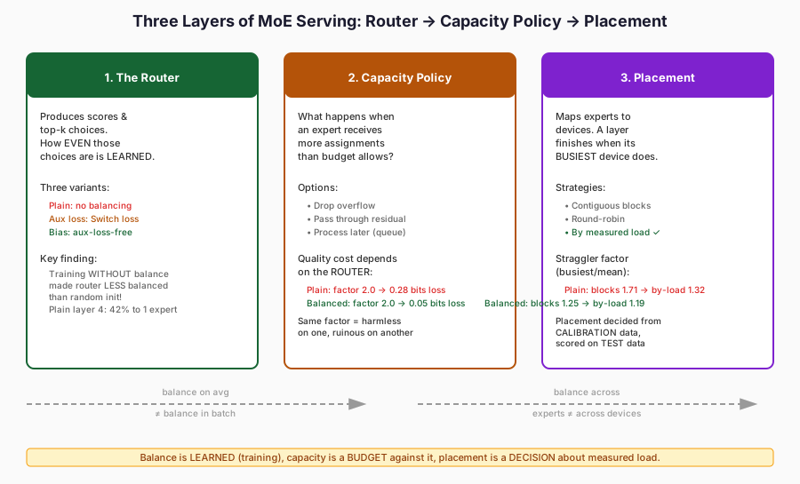
There are three distinct decisions. A router chooses experts and their weights; a capacity policy determines how to handle assignments that exceed the available slots; and placement maps experts to devices. The routing distribution affects the latter two, but neither follows automatically from a corpus-wide expert histogram. In this chapter the first decision is learned, the second is tested as an output mask, and the third is evaluated from assignment counts rather than measured multi-device execution.
- Routing: model scores and top-\(k\) selections determine which experts a token requests. Balance is evaluated from the resulting assignment counts, not inferred from the architecture.
- Capacity: a finite slot budget requires an overflow rule. The laboratory drops assignments in input order; other implementations can queue, reroute or execute them without dropping. A dropped contribution is skipped inside the MoE branch, while the transformer’s residual path remains.
- Placement: an expert-to-device map changes per-device assignment counts. Those counts proxy potential load imbalance, but actual execution time also depends on kernel efficiency, communication and overlap, none of which are directly benchmarked here.
A corpus can be well balanced even if individual dispatch groups are not; a device can be overloaded even when individual experts have similar average loads. I therefore report global assignment balance, group-wise overflow and simulated per-device assignment imbalance separately. Those observables answer related but different questions; the last is not a measured distributed straggler latency.
The laboratory
The laboratory model is a character-level transformer with four layers, model width \(d=192\), four attention heads, context length 128, and one top-2 MoE per transformer block. Each MoE contains 16 two-matrix GELU experts of hidden width 192, with a softmax over the selected router logits. The model contains 5,428,224 parameters. For every variant and seed (0, 1 and 2), the harness trains 2,000 AdamW steps on randomly sampled batches of 32 windows of 128 characters, with a 100-step warm-up and cosine learning-rate decay. The comparison changes the routing-balancing mechanism; it does not reproduce Mixtral’s gated expert architecture or the scale of the reference papers.
- Plain: top-2 selection with no auxiliary balancing objective or selection bias.
- Auxiliary loss: \(\alpha E\sum_i f_iP_i\) with \(\alpha=0.01\), where \(f_i\) is the fraction of top-2 assignments sent to expert \(i\), and \(P_i\) is its mean full-router softmax probability. The original Switch Transformer expression was developed for top-1 token dispatch. Here it is adapted to top-2 by dividing counts by the number of assignments, \(Tk\), rather than the number of tokens, \(T\). Because top-\(k\) selection is discrete, gradients flow through \(P_i\) rather than through the counts; the extra objective biases training toward more even load.
- Bias (auxiliary-loss-free): each expert has an additive bias used for top-2 selection, while the weights combined into the output are a softmax of the unbiased selected logits. Following each training forward pass, the bias moves by \(u\,\mathrm{sign}(\bar c-c_i)\), with \(u=0.005\) fixed in advance. The update is non-gradient and is disabled in evaluation mode. This is a small-model adaptation of the method described by Wang et al., not a reproduction of that paper’s scale or tuned settings.
The distinctions matter when comparing with the papers. Switch Transformers uses top-1 routing and a load-balancing term; the laboratory uses the same form of loss with a top-2 assignment frequency. Wang et al. describe the selection-only bias and a sign-based load update without an auxiliary gradient; here the step size is a predeclared local choice. DeepSeekMoE discusses additional expert- and device-level balancing objectives that the laboratory does not train. These papers motivate the mechanisms, while the measured quality and routing counts in this chapter are entirely local results.
Data and provenance. Training uses the manuscript text, Python examples and chapter tests for What Is Inference?–PagedAttention (739,076 characters in the recorded run); Continuous Batching–Prefix Caching form the 110,783-character calibration split used for placement, and Speculative Decoding–Compilation and Execution Graphs–Mixture-of-Experts Inference form the 227,957-character final evaluation split. A character vocabulary of 135 symbols is built from training data, with no unknown test characters in the recorded snapshot. Non-overlapping 128-character windows supply next-character predictions, so evaluation resets the model’s context at every window boundary. The splits are disjoint by chapter number, not necessarily by repeated phrases, common examples or duplicated code. Reproducibility hazard: corpus_split reads these files live. As the book is edited, the training and test datasets—and therefore the recorded 2.10-bit results—can change. Reproducing these figures requires the original repository commit or content hashes, the exact split manifest and seeds, not simply rerunning the script against the latest manuscript.
Unit tests compare the laboratory MoE with Mixture-of-Experts Inference’s reference computation: the unbounded forward gives equivalent outputs on a small random model, and the capacity-masked variant matches Mixture-of-Experts Inference’s explicit overflow-dropping dispatch, including assignment-drop counts. Further tests cover the bias update, load statistics, grouping and placement helpers. These are component-level functional checks; they do not verify the full nine-run GPU experiment, validate an actual sparse-kernel speed-up or establish large-model quality.
What the three variants do
Quality is reported first, as next-character bits per character on non-overlapping test windows. The table gives the mean and observed minimum–maximum across three training seeds; the calibration column is the mean score for the separate Continuous Batching–Prefix Caching split. These are descriptive measurements, not confidence intervals or an equivalence test.
| Variant | Test bits per character | Calibration |
|---|---|---|
| Plain | 2.104 (2.090 to 2.113) | 1.917 |
| Auxiliary loss | 2.103 (2.081 to 2.129) | 1.911 |
| Bias | 2.119 (2.103 to 2.133) | 1.926 |
The observed seed ranges overlap, so the experiment found no clear separation in held-out bits per character among the three variants. It did not establish that their population performance is equivalent: there are only three seeds, one corpus and no formal equivalence margin. The models also overfit: final training cross-entropy was roughly 0.8 nats per character (about 1.15 bits), compared with roughly 2.1 bits on the test split. That limits generalisation claims, although the test traces still document the routing distributions learned in this specific experiment.
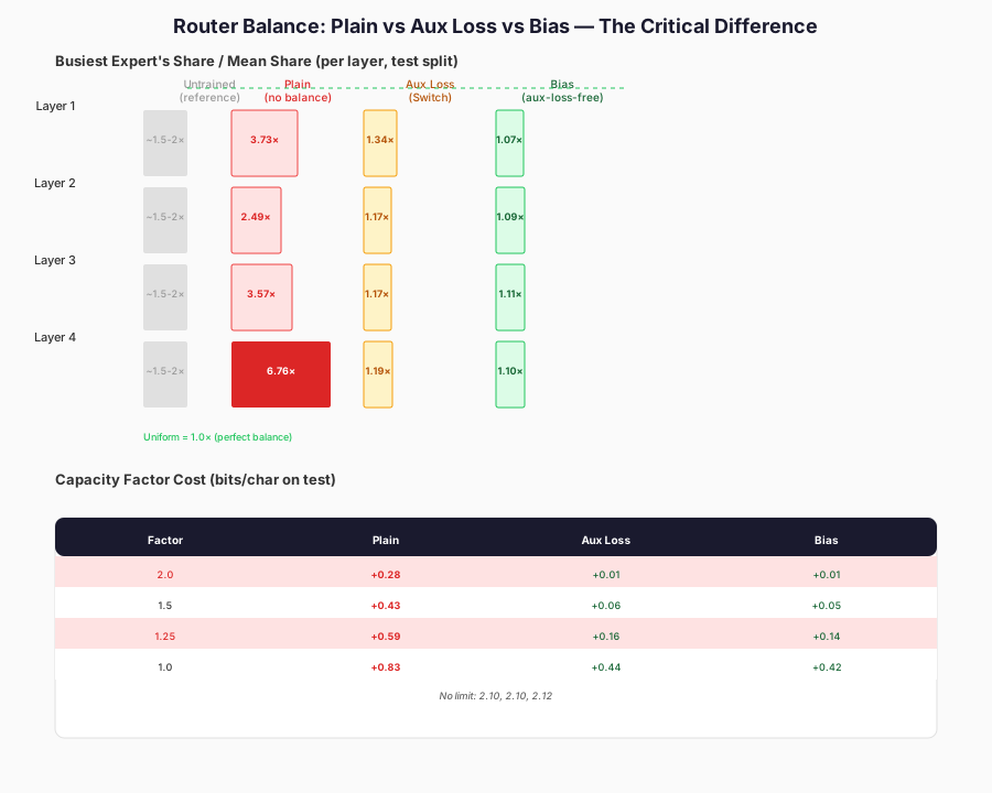
Routing balance is measured as \(\max_i c_i /(\sum_i c_i/E)\), the most-used expert’s assignment count divided by the mean count, aggregated over the test split. A value of 1 means equal totals, not equal per-batch loads. The table reports the three-seed mean by layer; the untrained row gives a range across three randomly initialised models.
| Variant | Layer 1 | Layer 2 | Layer 3 | Layer 4 |
|---|---|---|---|---|
| Untrained router (reference) | 1.4 to 1.6 | 1.5 to 1.9 | 1.8 to 2.8 | 1.6 to 2.2 |
| Plain | 3.73 | 2.49 | 3.57 | 6.76 |
| Auxiliary loss | 1.34 | 1.17 | 1.17 | 1.19 |
| Bias | 1.07 | 1.09 | 1.11 | 1.10 |
The unbalanced training runs concentrated assignments: the plain variant’s fourth layer gave its busiest expert an average of 42.3% of assignments, versus 6.25% under uniform top-2 assignment shares. Its busiest-over-mean ratio averaged 6.76 (across seeds, roughly 6.27–7.57) and routing entropy was much lower than uniform. The two balancing methods produced more even corpus-wide counts, with mean layer maxima of about 1.17–1.34 under the auxiliary loss and 1.07–1.11 under bias. This supports a mechanism-level conclusion for these models, not a general claim that unregularised MoE training always collapses. All experts had nonzero assignments on the test split, so strong concentration and complete expert inactivity are distinct outcomes.
The routers did learn something
An even expert histogram is not evidence that experts compute useful, different functions. As a more limited diagnostic, I measured the mutual information between the first-choice expert ID and a coarse category of the input character (letter, digit, space, newline or other). The implementation calls this nmi, but its precise normalisation is \(I(\text{expert};\text{class})/H(\text{class})\): it divides by character-class entropy, not a symmetric normalised mutual-information denominator. The result measures how predictive the routing choice is of character class. It does not by itself establish learned expert specialisation, causal usefulness of the expert choice or separation of semantic skills.
| Layer 1 | Layer 2 | Layer 3 | Layer 4 | |
|---|---|---|---|---|
| Untrained | 0.18 to 0.22 | 0.16 to 0.23 | 0.19 to 0.21 | 0.18 to 0.24 |
| Plain | 0.68 | 0.66 | 0.57 | 0.15 |
| Auxiliary loss | 0.65 | 0.62 | 0.63 | 0.50 |
| Bias | 0.59 | 0.62 | 0.55 | 0.46 |
The first three trained layers generally showed a larger expert-ID/character-class association than the three untrained reference networks, in this particular normalisation. The plain variant’s final layer scored only 0.15 on average, compared with 0.46–0.50 for the balanced variants; that is consistent with its concentrated first-choice routing reducing the diversity of the observed IDs. It is not evidence that balancing caused better semantic specialisation: token classes are a narrow proxy, the untrained models already show nonzero associations, and the sample contains just three seeds. A stronger test would measure expert ablations and the effects of changing routing at fixed weights, not only mutual information.
What a capacity limit costs
This experiment directly tests the quality consequence of overflow in Mixture-of-Experts Inference’s model, not its computational benefit. For each evaluation group of \(G\) tokens, each expert may contribute to at most \(C=\lceil cGk/E\rceil\) assignments, where \(c\) is the capacity factor, \(E=16\) and \(k=2\). Assignments beyond that capacity are masked out in input order; a skipped expert contribution is not added to the residual branch. Important implementation detail: MoEFFN.forward still computes the MLP output of every expert on every input token with dense einsum operations and then applies the routing/overflow mask. The run therefore measures changes to next-character loss, not reduced execution time, GPU weight traffic or memory use. The tables give test bits per character with the mean dropped share of expert assignments in parentheses, for groups of 512 tokens (four windows) and 64 tokens.
| Groups of 512 | Plain | Auxiliary loss | Bias |
|---|---|---|---|
| Factor 2.0 | 2.337 (20.1%) | 2.114 (0.7%) | 2.129 (0.8%) |
| Factor 1.5 | 2.529 (28.0%) | 2.159 (3.1%) | 2.164 (3.2%) |
| Factor 1.25 | 2.697 (33.5%) | 2.259 (6.7%) | 2.246 (6.7%) |
| Factor 1.0 | 2.935 (40.5%) | 2.538 (14.7%) | 2.537 (14.9%) |
| Groups of 64 | Plain | Auxiliary loss | Bias |
|---|---|---|---|
| Factor 2.0 | 2.388 (21.8%) | 2.151 (2.6%) | 2.162 (3.0%) |
| Factor 1.5 | 2.602 (30.2%) | 2.268 (7.3%) | 2.277 (7.8%) |
| Factor 1.25 | 2.781 (35.9%) | 2.440 (12.7%) | 2.451 (13.2%) |
| Factor 1.0 | 3.049 (43.1%) | 2.770 (21.7%) | 2.787 (22.3%) |
Compared with the no-limit scores of 2.104, 2.103 and 2.119 bits per character, factor 2.0 at groups of 64 increased the loss to 2.388, 2.151 and 2.162 respectively—about +0.285 bits for plain and +0.047/+0.044 for the balanced variants. At factor 1.25 the increases were approximately +0.677, +0.337 and +0.332 bits. The dropped shares follow the same ordering. Thus the same numerical capacity factor was far more damaging under these learned routing distributions. This supports choosing an overflow policy with knowledge of the model and workload. It does not show that any of these quality differences would become a particular speed-up under a truly sparse serving kernel.
Corpus-wide balance is not group-wise balance. Under the Mixture-of-Experts Inference independent, uniform top-2 selection model, the predicted drop fraction at factor 1.25 is about 0.084% for groups of 512 and 4.53% for groups of 64. The actual balanced models dropped about 6.7% and 12.7–13.2% respectively. Uniform marginal totals across the whole test corpus do not imply independent, uniform selections inside each group. The trace suggests local concentrations, but this experiment does not isolate whether code, prose, temporal correlation or another property causes them. Larger groups lower overflow for the balanced variants, while the unbalanced variant retains high losses because its busiest experts remain over-selected.
Capacity mitigation is a design choice, not an unavoidable drop-versus-padding binary. Reserving more slots lowers overflow but can increase padded work in a conventional fixed-capacity kernel; in the current laboratory implementation all expert outputs are already evaluated, so changing capacity alters the mask rather than the amount of expert arithmetic. An optimized engine could compact by expert, split overflowing assignments into a later pass, use a lossless grouped GEMM, or employ a different routing or admission strategy. Those options have different latency and memory costs and are not benchmarked here. Training-time balancing changes the distribution a runtime receives; it does not eliminate the need to check bursty loads.
Placement
Placement is evaluated as an assignment-count simulation, not as a multi-GPU run. For each layer and consecutive test window of 64 or 512 tokens, the score is the maximum device’s assigned-token count divided by the mean across four devices. The 16 experts are mapped four per device using contiguous IDs, round-robin IDs, or a greedy assignment based on expert counts measured on the separate calibration split. The replication variant adds two hot-expert copies and splits their assignment counts evenly. Scores are evaluated on the held-out test split. A simulated independent uniform top-2 router has an expected finite-window imbalance of about 1.18 at 64 and 1.06 at 512 tokens; these are reference expectations, not a physical lower bound on all possible placements or observed device completion times.
| Placement (windows of 64 / 512) | Plain | Auxiliary loss | Bias |
|---|---|---|---|
| Contiguous blocks | 1.75 / 1.71 | 1.34 / 1.25 | 1.31 / 1.20 |
| Round-robin | 1.90 / 1.87 | 1.32 / 1.22 | 1.33 / 1.22 |
| By calibration load | 1.39 / 1.32 | 1.29 / 1.19 | 1.28 / 1.17 |
| By load, plus 2 replicas | 1.41 / 1.37 | 1.30 / 1.21 | 1.30 / 1.21 |
For the plain variant, calibration-load placement reduced the test assignment-imbalance proxy from 1.71 to 1.32 at 512 tokens, approximately a 23% reduction. Round-robin gave 1.87 and was worse than contiguous placement for this particular learned routing pattern. The ordering differs from Mixture-of-Experts Inference’s index-ordered synthetic Zipf workload because the hot expert IDs here have no imposed ordering. The score computed on calibration traffic itself was about 1.33 for plain and 1.19/1.18 for the balanced variants, close to the held-out results in the recorded corpus. That is evidence for local stability of these assignment traces, not a measured 23% reduction in wall-clock layer time or a guarantee under workload drift.
The balanced variants began closer to even device counts; at 512-token windows, by-load placement reached about 1.19 and 1.17, compared with roughly 1.25 and 1.20 under contiguous placement. There is less headroom for placement to improve this count-based metric after training has spread assignments more evenly. In a real distributed system, expert execution costs need not be identical and communication can dominate, so the count proxy should be validated against actual per-device elapsed time before it drives deployment.
This replication heuristic did not help. Copying the two busiest calibration experts onto other devices, then assuming their traffic is split equally between the original and replica, increased the mean test imbalance proxy: for plain at 512 tokens, from about 1.32 to 1.37. The replica decision is fixed from calibration; the simulation does not allocate VRAM for the extra weights, route live requests, move weights or time communication. This is a negative result for this rule, not for replication generally. The pinned DeepInfer deployment Q&A describes redundant experts, measured rolling load and periodic reassignment, and reports slowest-rank-over-mean ratios of 1.045–1.090 on its authors’ systems. Those are vendor-reported results under different conditions, not a benchmark against this four-device simulation. The cited note should not be read as evidence of asynchronous weight transfers or a specific all-to-all schedule.
Communication
Distributing experts introduces two conceptually separate costs: shipping token activations to experts and returning their outputs, and waiting for the most heavily loaded device. For a simplified dispatch-plus-combine communication model, suppose each device originates \(t\) tokens, each token is sent to \(k\) distinct experts whose device placements are uniform and independent of the token’s origin, and the activation width is \(d\) values of \(b\) bytes each. A fraction \((D-1)/D\) of assignments then crosses devices on average. The resulting estimated outbound bytes per device, summing dispatch and return, is
| Tokens per device | 2 devices | 4 devices | 8 devices |
|---|---|---|---|
| 64 | 1.0 MB | 1.6 MB | 1.8 MB |
| 512 | 8.4 MB | 12.6 MB | 14.7 MB |
| 4,096 | 67 MB | 101 MB | 117 MB |
The only transfer rate measured locally is a pinned host-to-GPU copy: about 12.37 GB/s, versus about 12.66 GB/s in the reverse direction. Dividing the table’s bytes by 12.37 GB/s gives illustrative transfer times of 0.08–0.15 ms at 64 tokens per device, 0.68–1.19 ms at 512, and 5.43–9.50 ms at 4,096. This is not an all-to-all latency measurement, an inter-GPU bandwidth measurement or a lower bound on collective time. In particular, comparing the 64-tokens-per-device communication estimate with Mixture-of-Experts Inference’s 64-token-total, single-GPU layer time does not produce a valid 1–2% end-to-end overhead estimate: the effective batch sizes, execution geometry and potential overlap differ. Actual impact requires measuring an expert-parallel layer with the same batch definition, device placement, dispatch and interconnect.
Expert choice
Expert choice reverses the selection direction: for an available group of tokens, each expert selects its highest-scoring tokens, so it receives a fixed-sized bucket and a token may receive zero, one or many experts. I applied this selection rule to the token-choice-trained plain model’s second-layer routing probabilities for groups of 512 test characters, with 64 slots per expert. Each expert then received 64 tokens by construction; across the three recorded models, about 2.1–3.7% of tokens were assigned no expert and the largest number assigned to one token was 12. Only about 54.7–57.8% of assignments overlapped the model’s original top-2 token choices. This is a diagnostic of selection overlap and assignment shape, not a quality or throughput test of a model trained with expert choice. Expert choice needs the scores of the current dispatch group before it can allocate slots; it does not inherently require knowledge of tokens that have not yet been generated. For single-token online decoding, its capacity allocation and batching semantics differ from the multi-token groups measured here.
What the numbers do not show
- Small, overfitted model: 5.4 million parameters, characters rather than subword tokens, 16 experts per MoE and 2,000 training steps. No result generalises automatically to trained large MoEs.
- A live, evolving corpus: the harness builds the train/calibration/test text from the repository at run time. Edits to earlier book chapters or examples can change every measurement. The original commit or hashed snapshot must be retained to reproduce the published run.
- One chapter-based split: train (1–14), calibration (15–16), test (17–19) are disjoint source ranges, but repeated code or prose has not been audited for cross-split duplication.
- Three seeds only: overlapping quality ranges are not an equivalence test. Balance, association with character class and overflow vary across seeds.
- No evidence of semantic expert specialisation:
nmimeasures a specific conditional information fraction against five input-character classes, not whether experts acquired distinct useful skills. - Capacity is an output mask in this harness: every expert is computed for every input; latency, effective HBM reads and speed–quality trade-offs of true sparse capacity dispatch remain not measured.
- No physical expert-parallel execution: placement and replication use assignment counts; communication is volume arithmetic using host-device copy speed, not a measured all-to-all.
- Drop policy matters: the current rule keeps assignments in input order, not necessarily the most useful ones; no rerouting or overflow queue is implemented.
- Missing trained variants: no device-level balancing objective, sigmoid gating, shared experts or model trained with expert choice.
Inference Lab increment
The Lab now has:
build_model: character-level transformer withplain,auxandbiastop-2 MoE routing; dense expert evaluation and optional output-mask capacity limits.train_model,evaluate,collect_traces,windows: seeded training, non-overlapping 128-character evaluation windows, test and calibration traces; inputs are rebuilt from live files unless the corpus is frozen.load_balance_stats,nmi,bias_update: expert-count statistics, the explicitly normalised character-class association, and selection-only bias adjustment.place_block,place_round_robin,place_by_load,replicate_hottest,device_loads_from_counts,straggler: assignment-based placement and replication simulations.alltoall_bytes_per_device,expert_choice_mask: communication-volume arithmetic and an expert-choice mask, neither a distributed serving implementation.experiment,referenceandlinkcommands inexamples/ch20/routing_lab.py, with recorded observations inresearch/ch20/results.json.
The new inference rule is: learned routing defines demand, capacity changes the executed function if it drops assignments, and placement changes where that demand is served. These are separate controls. Before setting them for a deployment, measure the router on representative traffic, compare output quality under the intended overflow policy, and validate assignment-level estimates against real kernel and interconnect timings. A balanced global histogram is not enough, and the laboratory’s masked dense computation should not be mistaken for a measured sparse-serving speed-up.
What you should now be able to do
- Reproduce the Switch-style auxiliary loss as adapted here to top-2 assignment frequencies, and explain how it differs from the original Switch top-1 formula and from selection-only bias balancing.
- Calculate expert-load histograms, per-group drops and the exact \(I(\text{expert};\text{class})/H(\text{class})\) proxy without confusing it with semantic specialisation.
- Compare test bits per character with and without dropped assignments, and distinguish quality effects from unmeasured compute or memory savings.
- Build a calibration-based expert placement and evaluate its assignment-count imbalance on held-out traffic before claiming a runtime speed-up.
- Derive a per-device dispatch-and-combine byte estimate, state its assumptions, and avoid treating host-device copy bandwidth as inter-GPU collective performance.
- State the experimental limits of a small, overfitted, character-level model—and freeze a corpus snapshot before attempting replication.
Key terms
- Auxiliary balancing loss: a training objective that encourages an even assignment distribution; here a Switch-style expression adapted from top-1 to top-2 routing.
- Selection bias: an expert-specific score offset used in top-\(k\) selection and adjusted from load, without adding an auxiliary-loss gradient.
- Routing concentration: a high fraction of assignments going to a small subset of experts, whether or not any expert is completely unused.
- Capacity factor: multiplier applied to the average number of assignments per expert to obtain a finite slot budget.
- Dropped assignment: an expert contribution masked out when its allocated slots are exhausted; the residual stream remains.
- Character-class information fraction (
nmi): \(I(\text{expert};\text{character class})/H(\text{character class})\), an association proxy, not proof of semantic specialisation. - Placement: assigning expert weights and traffic to devices; here modelled by assignment counts only.
- Straggler ratio: busiest device’s assigned load divided by average assigned load, not necessarily its elapsed-time ratio.
- Expert replica: another copy of an expert’s weights that can split demand, at a memory cost not included in this experiment.
- Expert-choice routing: experts select tokens from an available group rather than each token selecting a fixed number of experts.
Reader exercises
- Freeze the exact What Is Inference?–Mixture-of-Experts Inference source snapshot and split-file hashes before rerunning
experiment. Does the recorded 739,076/110,783/227,957-character corpus reproduce after editing this book? - Tune the bias update rate \(u\) on calibration data alone, then report the test results once. Separate the effect of training randomness from the choice of update rate.
- Implement a genuinely sparse, lossless grouped dispatch and compare its latency and bytes moved with the current dense-all-experts-and-mask forward at capacity factors 1.0, 1.25 and no drop.
- Replace the earliest-assignment overflow rule with highest-gate-weight retention. Compare drop fractions and held-out bits per character on the same fixed test trace.
- Use per-layer expert ablations or forced routing changes to test whether the observed character-class association predicts causal expert specialisation.
- Implement DeepSeekMoE’s device-level balancing objective and train four-device groups, without selecting hyperparameters on the test split.
- Refit placement on a drifting calibration workload and score a later, all-code workload; compare assignment imbalance with actual multi-device execution times if hardware permits.
- Improve the replication heuristic using calibration counts and include its extra weight memory and any copying or communication cost.
- Benchmark expert-choice selection on the currently available decode batch, not on future tokens, and train a model specifically for that policy before comparing quality.
- Repeat the communication model for real GPU-to-GPU bandwidth and startup latency, using the same tokens-per-device definition as the compute benchmark.
References
- Switch Transformers: Scaling to Trillion Parameter Models with Simple and Efficient Sparsity — Fedus, Zoph and Shazeer, Journal of Machine Learning Research 23 (2022). Primary source for top-1 dispatch, expert capacity and its auxiliary balancing loss; the book adapts the loss to top-2 assignments.
- Auxiliary-Loss-Free Load Balancing Strategy for Mixture-of-Experts — Lean Wang et al., 2024 preprint. Primary source for selection-only expert bias and load-driven sign updates; this chapter uses a separately chosen update rate and a far smaller model.
- DeepSeekMoE: Towards Ultimate Expert Specialization in Mixture-of-Experts Language Models — Dai et al., ACL 2024. Context for fine-grained experts and expert-/device-level balancing; the laboratory does not reproduce its architecture or performance.
- Mixture-of-Experts with Expert Choice Routing — Zhou et al., NeurIPS 2022. Experts select their token buckets; the local
expert_choice_maskis only a selection-rule illustration. - DeepInfer inference deployment Q&A, pinned at commit 774ce244 — first-party vendor design note on redundant experts and reassignment. Author-reported load ratios are not reproduced here, and no undocumented transfer mechanism is inferred.
Evidence in this chapter
| Claim | Evidence category and limit |
|---|---|
| Switch auxiliary loss, Wang’s selection-only bias, DeepSeekMoE device balancing, expert-choice design | Established background, cited primary publications; local top-2 and update-rate adaptations identified |
| Plain, auxiliary and bias models scored 2.104, 2.103 and 2.119 bits per character | Book result, three seeds and one character-level test split; no equivalence test |
| The plain model reached 6.76 times mean expert load in layer 4; balanced variants were much more even | Book result, aggregate expert assignments across this toy model’s test split |
| First-choice expert IDs were associated with character class (roughly 0.55–0.68 versus 0.2 untrained in early layers) | Book result for the specific \(I/H(\text{class})\) diagnostic; semantic specialisation not established |
| At group size 64 and factor 2.0, overflow increased test loss by about 0.285 versus 0.044–0.047 bits/character | Book result of dropping assignments from a dense-all-experts evaluation path; no serving speed-up measured |
| Uniform independent routing predicts 0.084% drops at group 512 and factor 1.25, versus about 6.7% observed | Analytical baseline plus local count measurements; independence assumption not satisfied by learned routing |
| Calibrated placement reduced the 512-token plain-model assignment straggler proxy from 1.71 to 1.32 | Book result of a held-out assignment-count simulation, not distributed elapsed time |
| Replicating two hot experts worsened that proxy in the chosen heuristic | Local simulation only; no replica memory or network accounting |
| DeepInfer reports redundant-expert deployment and slowest-rank/mean ratios around 1.045–1.090 | Vendor-reported facts from pinned documentation, not locally verified |
| Table of dispatch and combine byte volumes based on 12.37 GB/s host-device copy | Arithmetic illustration, not measured all-to-all or comparable total distributed latency |
| Sparse serving performance, semantic expert specialisation, large trained MoEs and drifting production traffic | Not measured |
| Source reproducibility across book revisions | Not yet qualified: corpus is assembled from mutable manuscript, examples and tests; source snapshot should be pinned |