Probabilities, Logits, and Soft Targets
A teacher's final layer returns scores, not certainties. This chapter derives softmax, temperature scaling, cross-entropy, and the logit gradient, then connects them to the tested E1 implementation.
Give a softmax written directly from its textbook formula the three numbers \((1000, 999, 998)\) and it returns not-a-number. Give it \((2, 1, 0)\) and it returns \((0.6652, 0.2447, 0.0900)\). Yet the two inputs describe exactly the same distribution, and a stable implementation returns those same three probabilities for both. The numbers a classifier produces are not probabilities; once they pass through a softmax, only their differences matter; and how they are turned into a distribution is a design decision with numerical consequences.
Chapter 03 chose a teacher and a student. This chapter examines the signal that passes between them. A classifier’s final layer does not return a probability directly. It returns a vector of real-valued scores, and the meaning of those scores depends on how they are normalised. Temperature changes that normalisation. Cross-entropy turns a target distribution and a predicted distribution into a loss. The gradient of that loss with respect to the logits has a simple and useful form.
These are the mathematical ingredients of distillation. They are also ordinary classification mathematics. The distillation-specific question is what happens when the target distribution is supplied by a teacher rather than by a hard label.
The central question is:
What information does a teacher’s output distribution contain, and how does temperature change it?
The chapter answers that question in steps: logits, softmax, temperature, soft targets, cross-entropy, gradients, numerical stability, and the limits of the “dark knowledge” interpretation. E1 supplies the implementation and a warning against assuming that a richer target is automatically a better target.
Logits are scores, not probabilities
A classifier with \(K\) classes produces a vector
A hard label is a single target class or token. For a \(K\)-class problem, it is often written as an integer \(y \in \{0,\ldots,K-1\}\), or as a one-hot vector \(q\) with \(q_y=1\) and \(q_i=0\) for \(i \ne y\). This matches the zero-based class indices used by PyTorch and E1. The hard label says which class is correct. It does not say that another class was plausible, that two classes are similar, or that the example is ambiguous.
A soft label is a probability distribution \(q=(q_1,\ldots,q_K)\) with \(q_i \ge 0\) and \(\sum_i q_i=1\). It may come from a teacher, from label smoothing, from an ensemble, or from another target-construction process. A soft label is not automatically ground truth. It is a target distribution with a source and a provenance.
The distinction matters because a hard label and a soft label answer different questions. The hard label says “choose class \(y\).” A soft label says “allocate probability mass across the classes in this way.” The second can carry more information, but it can also carry the teacher’s errors, biases, or overconfidence. A hard label is not a defective soft label; it is a different target with less information and often a stronger correctness guarantee.
A teacher prediction is not ground truth, and label smoothing is not the same thing as a teacher prediction. Label smoothing constructs a target from the label; a teacher constructs a target from its learned behaviour. Both can produce soft targets, but their provenance and failure modes differ.
From scores to probabilities
The standard way to turn logits into a probability distribution is the softmax function:
The softmax also has a useful odds interpretation:
Positivity and sum-to-one are necessary properties of a probability distribution, but they do not uniquely determine softmax. Any positive vector that sums to one is a valid distribution. Softmax is a particular modelling choice among normalisations of the form \(p_i\propto f(z_i)\): an exponential scoring rule that preserves the ordering of the logits and makes the log-odds linear in logit differences. The exponential is not the only possible normalisation, but within that class it is the one that turns additive logit differences into the log-odds \(\log(p_i/p_j)=z_i-z_j\). That is why logits can be treated as additive evidence in a multi-class model.
Example A — From logits to probabilities
Take the three logits
Temperature changes the distribution
Temperature is a positive scalar \(T\) applied by dividing the logits before softmax:
- As \(T \to 0^+\), let \(M=\max_i z_i\) and let \(A=\{i:z_i=M\}\). The probability on each class in \(A\) approaches \(1/|A|\), and the probability on every other class approaches zero. If the maximum is unique, the limit is a one-hot distribution. If several logits tie at the maximum, the limit is uniform over the tied classes, not a single class.
- As \(T \to \infty\), every \(z_i/T\) approaches zero, so every numerator approaches one and \(p_i \to 1/K\). The limit is the uniform distribution.
Temperature must be strictly positive. \(T=0\) is not a valid setting; it is a limit, not a value the implementation should accept. The E1 loss code validates that temperature is finite and positive.
For a fixed finite logit vector, entropy is non-decreasing as temperature increases. The entropy of a distribution \(p\) is
Example B — Three temperatures
Use the same logits \(z=(2,1,0)\). The probabilities and entropies are:
| Temperature | Probabilities | Entropy |
|---|---|---|
| \(T=1\) | \((0.6652,\ 0.2447,\ 0.0900)\) | \(0.8324\) |
| \(T=2\) | \((0.5065,\ 0.3072,\ 0.1863)\) | \(1.0202\) |
| \(T=10\) | \((0.3672,\ 0.3322,\ 0.3006)\) | \(1.0953\) |
The uniform distribution on three classes has entropy \(\log 3 \approx 1.0986\). At \(T=10\), the distribution is close to uniform but not identical to it. The entropy increases from \(0.8324\) to \(1.0202\) to \(1.0953\), consistent with the derivative above.
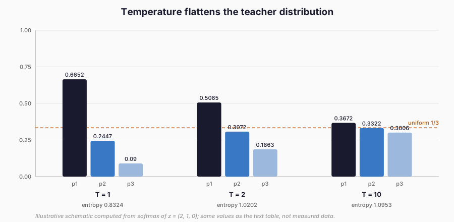
Figure 1. The three rows of the table above, drawn as bars. Higher temperature moves mass from the top class to the others; at \(T=10\) the bars approach the uniform line. Illustrative schematic computed from the softmax formula, not measured data.
The table is illustrative, not an E1 measurement. The values were computed from the formula and checked against the implementation at double precision.
Soft targets and what they can carry
A soft target assigns probability mass to more than one class. For a three-class problem, a teacher might produce
The phrase dark knowledge is sometimes used for the information in the non-target probabilities. The phrase is a metaphor, not a substance inside the model. There is no separately measurable quantity called dark knowledge. There is a distribution, and the distribution may contain useful structure, noise, or both. The next section measures prediction error against such a distribution.
Cross-entropy measures the target mismatch
Cross-entropy between a target distribution \(q\) and a model distribution \(p\) is the registered \(L_{\mathrm{CE}}\),
For a hard label \(y\), the target is one-hot: \(q_y=1\) and all other entries are zero. The sum collapses to one term:
A useful lower bound is that, for a fixed target \(q\), the smallest possible cross-entropy over distributions \(p\) is the entropy of \(q\), attained when \(p=q\). For a hard label, that entropy is zero; a finite softmax approaches zero as the correct logit dominates. For a non-degenerate soft target, \(L_{\mathrm{CE}}(q,q)=H(q)>0\): even a model that matches the target exactly has a positive loss. Chapter 05 uses this fact when it decomposes the distillation objective.
Example C — Hard and soft cross-entropy
Use \(p=(0.6652,0.2447,0.0900)\) from Example A.
For the hard target \(q=(1,0,0)\),
The gradient has a simple form
Let \(L=L_{\mathrm{CE}}(q,p)\) with \(p=\operatorname{softmax}(z)\). The derivative of the softmax is
If the logits are temperature-scaled, \(u_i=z_i/T\), then
The gradient formula was checked against PyTorch autograd in the focused tests, and the KL gradient was additionally checked with an independent central finite-difference calculation. A central finite-difference check perturbs one logit by \(\pm\epsilon\), recomputes the loss on both sides, and compares \((L(+\epsilon)-L(-\epsilon))/(2\epsilon)\) with the analytic derivative. The tests use double precision and a tolerance of \(10^{-12}\) for the analytic comparison.
Numerical stability
A naive softmax computes \(e^{z_i}\) directly. For large positive logits, the exponential overflows; for large negative logits, it underflows to zero and the denominator may become zero. Neither case is acceptable.
The stable identity subtracts the maximum logit before exponentiating. Let \(m=\max_i z_i\). Then
The log-domain version is
PyTorch’s torch.softmax and torch.log_softmax are documented to be computed
in a numerically stable way; the implementation here relies on that documented
behaviour and the focused tests check finite outputs for the expected range.
The chapter still derives the identity because the reader should know what the
library is doing, and because a naive implementation in another language or on
another array type can fail.
Example D — When naive exponentiation fails
Take \(z=(1000,999,998)\). A naive implementation evaluates \(e^{1000}\), which overflows to infinity in ordinary floating point; dividing infinity by infinity produces not-a-number. The stable form subtracts \(m=1000\), evaluates \((e^0,e^{-1},e^{-2})\), and produces the same probabilities as Example A: \((0.6652,0.2447,0.0900)\).
Take \(z=(-1000,-1001,-1002)\). A naive implementation evaluates three exponentials that underflow to zero, leaving \(0/0\). The stable form subtracts \(m=-1000\), evaluates \((e^0,e^{-1},e^{-2})\), and again produces the same distribution. The absolute logits were extreme; their differences were not.
For log-probabilities, the direct log_softmax path avoids forming a probability
that may underflow before the logarithm. A naive log(softmax(z)) can lose
precision or produce negative infinity when the probability underflows; the
stable log-domain form keeps the finite logit differences.
No numerical method guarantees arbitrary precision for every dtype or every input. The implementation should validate finite inputs where the interface allows it, use an appropriate dtype, and test the range it actually expects. The chapter’s hand examples use double precision; the code tests use tolerances appropriate to the dtype.
What dark knowledge can and cannot justify
The useful intuition behind soft targets is that a teacher may assign non-target mass in a meaningful pattern. If a teacher gives \(0.70\) to class A, \(0.25\) to class B, and \(0.05\) to class C, the relative mass suggests that B is closer to A than C is. A hard label would discard that pattern. Hinton et al. (2015) used this intuition to motivate temperature-scaled soft targets.
The intuition has limits:
- The teacher may be overconfident, so the non-target mass may be tiny.
- The teacher may be wrong, and the student can learn the error.
- The similarity structure may be incorrect or irrelevant to the task.
- A large capacity gap may make the teacher’s distribution hard for the student to use.
- Distribution shift can make the teacher’s behaviour misleading.
- A soft target can improve calibration while leaving accuracy unchanged or worse; the metrics answer different questions.
- The teacher forward pass, storage, and hyperparameter search add cost.
Müller et al. (2019) provide a useful caution. They report that label smoothing can improve calibration, but that a teacher trained with label smoothing can be less effective for distillation because its logits lose information about resemblances between classes. A softer target is not automatically a more informative one. The shape of the distribution matters, not merely its entropy.
E1 is the bounded demonstration. The mixed-distillation student had lower cross-entropy and lower measured calibration error than the hard-label baseline, but also lower mean held-out accuracy. The dark-knowledge argument cannot overrule that result. It can motivate a hypothesis; the held-out task decides whether the hypothesis is useful.
Distillation temperature is not calibration temperature
Temperature appears in at least two different practices:
- Distillation temperature: during training, the teacher and student logits are divided by \(T\) so the teaching distribution is softer and the student can learn from relative probabilities.
- Post-hoc calibration temperature: after training, a temperature may be selected on held-out data to adjust predictive confidence.
The mathematical transformation is similar, but the objective is different. A distillation temperature shapes a training target. A calibration temperature adjusts a deployed model’s confidence. A softer distribution is not necessarily a better-calibrated one. Calibration must be measured on held-out data, and a temperature selected for one purpose should not be assumed to serve the other.
Chapter 05 uses temperature in the distillation objective. Chapter 34 develops calibration measurement. This chapter uses temperature only to explain the distribution.
The E1 implementation
The E1 code already contains the relevant functions in
examples/common/losses.py:
| Function | Role |
|---|---|
softmax(logits, temperature=1.0) |
Divides logits by temperature, then applies torch.softmax |
log_softmax(logits, temperature=1.0) |
Divides logits by temperature, then applies torch.log_softmax |
temperature_scale(logits, temperature=1.0) |
Alias for softmax in the E1 API |
cross_entropy(logits, targets, reduction="mean") |
Hard-label cross-entropy via F.cross_entropy |
soft_cross_entropy(logits, targets, reduction="mean") |
Soft-target cross-entropy over a normalised target distribution |
entropy(logits) |
Mean entropy of the softmax distribution |
A teacher/student calculation can be expressed as:
from examples.common.losses import (
    cross_entropy,
    log_softmax,
    soft_cross_entropy,
    softmax,
)

teacher_probs = softmax(teacher_logits, temperature=2.0)
hard_loss = cross_entropy(student_logits, targets)
soft_loss = soft_cross_entropy(student_logits / 2.0, teacher_probs)

# log p_S at T = 2; Chapter 05 uses this inside the KL term.
student_log_probs = log_softmax(student_logits, temperature=2.0)
The soft_loss here is a raw cross-entropy against the temperature-scaled
teacher distribution. It is not the complete distillation objective. Chapter 05
derives the KL term and the \(T^2\) compensation that E1’s distillation_loss
uses. The existing E1 mixed loss is unchanged.
soft_cross_entropy is new in this chapter and is not used by the E1 training
path. It validates that the target has the same shape as the logits, is finite,
non-negative, and sums to one along the class dimension. Focused tests cover the
one-hot equivalence, the uniform-target value, the \(p-q\) gradient, the
temperature chain rule, and invalid target shapes or normalisation.
The E1 teacher and student logits are four-dimensional vectors. softmax and
log_softmax operate on the last dimension, so each example in a batch is
normalised independently. The hard arm calls cross_entropy; the mixed arm calls
distillation_loss, which uses kl_divergence internally. The new
soft_cross_entropy helper is used for the chapter’s soft-target checks, not for
E1 training. This keeps the frozen E1 path unchanged while making the soft-target
mathematics testable in isolation.
The same functions apply to any batch of vectors with a class dimension; the batch dimension is independent of the softmax.
Rights are part of the signal
Probabilities and logits are still model outputs. They can be subject to service terms, output-use restrictions, confidentiality obligations, personal-data rules, and training-data permissions. Whether a returned probability vector counts as “Output” under a competing-model clause is an open interpretive question for specialist review; the OpenAI Services Agreement, for example, restricts using outputs to develop competing models (L-016; retrieved 12 November 2026), and that reading should not be assumed to cover or exclude every numeric return without checking the current terms. A teacher’s outputs may also contain user data or reproduce protected material. The fact that the values are “only numbers” does not make them unrestricted.
E1 uses self-created data and models under RM-101, and the numeric examples in this chapter are synthetic. Chapters 36–39 develop the legal framework; this chapter treats outputs as data with provenance, not as automatically safe artefacts.
Limits of this chapter’s evidence
Almost every number in this chapter is illustrative arithmetic: Examples A–D, the three-temperature table, and the cross-entropy and gradient values were computed from the formulas and checked against the implementation at double precision. None of them is an E1 measurement. The one book result the chapter uses is E1’s mixed student having lower cross-entropy and lower measured calibration error alongside lower mean accuracy, on one synthetic task with three seeds. The derivations are established background. “Dark knowledge” is a metaphor, not a measured quantity, and the label-smoothing caution is the finding Müller et al. (2019) report. Whether a returned probability vector counts as “Output” under a service’s terms remains an open question for specialist review.
What comes next
The pieces are now explicit: logits become probabilities through softmax; temperature changes the distribution; soft targets are distributions; cross-entropy measures mismatch; its gradient is \(p-q\). Numerical stability is a property of the implementation, not a different objective.
Chapter 05 combines these pieces into the distillation objective. It derives the KL term, explains why the teacher and student distributions are compared at the same temperature, and shows why the \(T^2\) factor appears. The result is the objective that E1 already implements and that the later chapters extend.
References
Hinton, G., Vinyals, O. and Dean, J. (2015). Distilling the Knowledge in a Neural Network. NIPS 2014 Deep Learning Workshop. arXiv:1503.02531. https://arxiv.org/abs/1503.02531
Müller, R., Kornblith, S. and Hinton, G. (2019). When Does Label Smoothing Help? Advances in Neural Information Processing Systems. arXiv:1906.02629. https://arxiv.org/abs/1906.02629
Legal sources
OpenAI Services Agreement. Updated 1 December 2025; effective 1 January 2026. https://openai.com/policies/services-agreement/ (retrieved 12 November 2026).