Parameter-Efficient Distillation
Can a student acquire teacher behaviour while updating far fewer parameters? LoRA adapters on a frozen base, a two-point rank sweep, exact merging, and a clean negative: with a random frozen base, the adapter fails where full fine-tuning succeeds.
Chapter 31 chose among students by measured deployment cost and found that distillation never changes the price tag: a student’s architecture fixes its cost, and that choice is made before training starts. This chapter asks the complementary question. Suppose training itself is the scarce resource — optimiser memory, update budget, the number of weights you may touch — while deployment cost is fixed. Can the student acquire the teacher’s behaviour while updating far fewer parameters?
Can a student acquire teacher behaviour while updating far fewer parameters, and what trade-offs does that introduce?
The measured answer is a clean negative with an exact merge. Full fine-tuning reaches 0.400 functional correctness; LoRA at rank 4 reaches 0.023; rank 1 reaches 0.000 with fully invalid outputs; a smaller fully trained model reaches 0.093. Merging is exact up to fp32 rounding (max difference ~1e-6) and buys ~9% latency. The adapter cuts optimiser memory 5.8-fold — and loses the task, inflates the checkpoint, and leaves inference latency no better than full fine-tuning’s.
The reason is stated plainly and early, because it conditions everything: the frozen base here is randomly initialised, not pretrained, so the comparison measures parameter-efficient training from scratch, not adaptation of a competent base. Production LoRA adapts models that already work; ours adapts noise. The structural findings — what trainable counts do and do not buy — survive that qualification. The capability ranking does not transfer beyond it, and the chapter says so where it matters instead of once in small print.
Full fine-tuning, frozen bases, and the adapter idea
Full fine-tuning updates every weight: given a loss \(L\), each parameter \(W\) moves by \(-\eta \nabla_W L\), and Adam keeps two running moments per parameter — eight bytes of optimiser state per trainable fp32 weight, before counting the weights themselves or the activations. A frozen base updates nothing: its gradients are never computed, its optimiser state is never allocated.
An adapter splits the difference — most weights frozen, a small trainable appendage carrying the entire update — so optimiser memory scales with the appendage while the forward pass still pays for the whole model. That asymmetry (cheap to optimise, full price to run) is the whole economic content of parameter-efficient methods, and every claim about them should be checked against it.
Low-rank adaptation (Hu et al., P-048) makes the appendage a factorised update to an existing matrix. For a frozen base map \(W_0 \in \mathbb{R}^{d_{\mathrm{out}} \times d_{\mathrm{in}}}\),
The forward pass is \(y = W_0 x + (\alpha/r) B(Ax)\): the frozen path plus a low-rank correction. Gradients flow to \(A\) and \(B\) through the frozen \(W_0\) without ever updating it — autograd differentiates through constants cheaply, and the base weights are constants by construction (frozen before the first step, asserted unchanged after training by direct comparison in the test suite).
The teacher signal reaches the adapters the same way: mixed KL at the output distribution produces output gradients, which backpropagate through frozen layers down to every factor. No per-layer teacher signal is needed — unlike FitNets-style feature matching, which would require aligned intermediate targets, the output distribution alone supervises all sites through the chain rule. That is a property of the objective’s placement (at the head), not of adapters generally: move the distillation loss to an intermediate layer and the factors above it would starve, a configuration the study does not run and the chapter does not recommend blind.
Parameter arithmetic follows from the shapes. One adapted \(m \times n\) matrix costs \(r(m+n)\) trainable parameters against \(mn\) frozen ones. Our student wraps three sites per transformer block — attention out-projection (\(16\times16\)) and both MLP matrices (\(16\times64\), \(64\times16\)) — at rank 4: \(4(16+16) + 4(16+64) + 4(64+16) = 128 + 320 + 320 = 768\) trainable parameters on a 4,464-parameter base (5,232 total deployed). At rank 1 the same sites cost \(32 + 80 + 80 = 192\). Rank is capacity in the most literal sense: the update \(\Delta W = (\alpha/r)BA\) has rank at most \(r\) no matter what the task needs, and no optimiser, budget, or scaling factor raises it.
Geometrically, rank 1 is a single outer product — every row of the update is a multiple of one vector, so the adapter can shift behaviour along one direction only. Our D arm lives there (192 parameters) and scores exactly 0.000 with fully invalid outputs: rank starvation made visible, not hypothesised. Rank 4 allows four independent directions and scores 0.023 — better in the only sense available at the floor (some template, no sums). The sweep is two points, and the chapter refuses to fit a curve through them: what two points establish is that rank matters and that neither rank suffices here, which is a bound on the claim, not a scaling law.
What the ledger actually records
Four ledgers, four different answers. Trainable parameters (768 vs 4,464) measure optimiser state and update bandwidth: Adam needs \(8\) bytes per trainable parameter (first and second moments in fp32), so B-r4 books 6,144 bytes against A’s 35,712 — a 5.8-fold saving, the single clear win, and the only one. Total parameters (5,232 vs 4,464) measure what ships and what runs: the adapter student deploys MORE weights than the full student, because the base stays and the factors add. Checkpoint bytes agree (20,928 vs 17,856): the “efficient” student’s artefact is 17% larger.
Training wall time is roughly tied (~9.6 vs ~10.0 s per seed for 600 matched updates): the frozen base still forwards every batch, and forward passes dominate at this scale. Inference latency is tied with arm A within run-to-run noise. Merging the adapter is ~9% faster than leaving it unmerged on every seed (seed 50: 1.313 → 1.197 ms per 32-row batch) — the merge removes the two extra matmuls per site, and the measurement, not the parameter count, says how much that is worth here: 0.1 ms.
The mission’s strategic distinction runs through every row: a student that saves 83% of trainable parameters but ships 17% more weights, trains for the same wall time, and infers no faster has not demonstrated deployment efficiency. It has demonstrated a cheaper optimiser state. Whether that matters depends on what is scarce — GPU memory for Adam moments, say, or update bandwidth to the field — and the chapter’s contribution is the ledger that lets the reader decide, not the decision.
The frozen E3 comparison
Same JSON-sum task and splits as the frozen E3-structured study (fingerprint-verified identical before any training), fresh w32/L2 teacher retrained under a new run ID (validation 0.890 / 0.910 / 0.915, gate cleared), four w16-family students at EXACTLY 600 matched updates with seed-matched inits where architectures match, mixed KL (\(\lambda = 0.5\), \(T = 2.0\)) throughout:
| Seed | A-full | B-r4 | D-r1 | C-small |
|---|---|---|---|---|
| 50 | 0.405 | 0.068 | 0.000 | 0.110 |
| 51 | 0.378 | 0.000 | 0.000 | 0.113 |
| 52 | 0.417 | 0.000 | 0.000 | 0.058 |
Aggregates: A 0.400 ± 0.020, B 0.023 ± 0.039, D 0.000 ± 0.000, C 0.093 ± 0.031. Token accuracy tells the same story one level down: A 0.91, B 0.80, D 0.29, C 0.83 — B learned the template (four of five tokens right) and almost none of the arithmetic; D, with invalid outputs on every test input (invalid rate 1.000), learned not even the template. Numerical precision is fixed throughout at
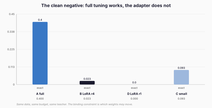
Figure 1. Held-out functional correctness per arm: the full model at 0.400, the smaller full model at 0.093, the adapters at 0.023 and 0.000. Same data, same budget, same teacher. Frozen E3S measurements. fp32 — weights, factors, optimiser moments, merged equivalents — so no result here depends on a dtype the chapter did not measure. A bf16 repeat would halve the checkpoint bytes and change the merge rounding from ~1e-6 to ~1e-3 territory; it would not change which arm learns, and the chapter leaves the dtype sweep unrun rather than asserting that.
Three readings. H1 holds: full fine-tuning beats the rank-4 adapter on all seeds (+0.337 / +0.378 / +0.417 — attributable to which parameters may move, since everything else is matched at the single shared learning rate). H2 holds at the floor: r=4 (0.023) beats r=1 (0.000) — rank matters, and both fail, which bounds the sweep’s informativeness honestly: a two-point sweep distinguishes “fails less” from “fails”, not a scaling law. H3 is measured, not ranked: the smaller full model (1,464 params total, all trainable; 0.093) beats the LoRA student (768 trainable of 5,232 total; 0.023). Neither trainable count (1,464 > 768) nor total capacity (5,232 > 1,464) predicts the ordering. The likeliest explanation is the frozen random base: C’s 1,464 parameters all learn, while B’s 768 learn around 4,464 frozen random ones.
On that reading, the binding constraint is which weights may move, not how many. The chapter states it as a mechanism hypothesis, consistent with the numbers but untested here (the trained-base ablation below is the test), with the random-base qualification attached. C is also the honest baseline the mission asked for: smaller, fully trainable, no base to inherit and no adapter to merge — redistributes cleanly, trains anywhere, and still fails the task (0.093). When the choice is between a small model that fails plainly and an adapter that fails while borrowing a base it cannot ship without, the ledger prefers the plain failure.
That is not an endorsement of C; it is the form the comparison should take. As guidance rather than verdict: pick the small full model when there is no competent base to borrow, when redistribution must be clean, or when training anywhere matters more than optimiser memory. Pick the adapter when a competent base exists, the task varies on what the base already does, and optimiser memory or update bandwidth is the binding constraint — the three conditions this study violates by design (random base, new task, tiny budgets) and production LoRA satisfies by premise. The ledger does not choose for you; it shows which premise you are buying.
Why the adapter fails here (and what that does and does not show)
The honest mechanism runs through the initialisation. Production LoRA (P-048’s GPT-3/RoBERTa results: up to 10,000× fewer trainable parameters, on par or better quality) adapts a pretrained base whose frozen weights already implement the task’s prerequisites; the factors steer competence that exists. Our base is random: its frozen weights implement nothing, so the factors must build the behaviour from scratch through a rank-4 bottleneck — 768 parameters asked to do the work that 4,464 do in arm A, with the optimiser denied access to the other 4,464.
The failure (0.023 vs 0.400) is therefore a finding about PEFT-without-pretraining, and the chapter refuses to promote it into a verdict on production LoRA, where the premise is reversed. What does transfer: the accounting identities (trainable vs total vs optimiser vs checkpoint), the merge exactness, the rank ordering at the two points measured, and the warning that adapter papers’ headline ratios (“10,000× fewer parameters”) describe trainable parameters only. Their GPT-3 claim is theirs, cited as background and not replicated; our 83%-fewer-trainable claim is ours, measured, and accompanied by the totals that qualify it.
Two ablations the study does not run, and one gap built into its design, recorded so their absence is visible. First, LoRA on a trained base (freeze arm A’s final weights, then distil further into adapters): the direct test of whether the failure is the random base or the adapter form, omitted for budget discipline, not for lack of interest — and the single most informative follow-up, since a positive there would localise tonight’s negative to initialisation rather than to adapters as such.
Second, rank 8/16 and more sites (attention QKV, embeddings): the sweep stops at r=4 because r=1 already floors, but a higher-rank arm could in principle recover — unmeasured, hypothesised, not claimed. The contract’s rank sweep is satisfied as a two-point comparison with the bound stated, not as a scaling study. Third, implicit in the design: interference across tasks is untested because there is one task; a shared adapter serving two distributions would need conflict metrics (gradient alignment, per-task deltas) this study has no second distribution to compute.
Merge, unmerge, and the latency that isn’t there
Merging replaces each LoRA site with its fused dense equivalent: \(W_{\mathrm{fused}} = W_0 + (\alpha/r)BA\), computed once, exactly — algebraically identical, with only floating-point rounding between the two forms (measured ~1e-6 here, within the test suite’s 1e-5 bound on hand-built modules). Unmerge is free and perfect — the base was never modified, so “unmerging” is just keeping the base. Make that a habit, not a footnote: every adapter run in this book henceforth keeps the unmerged base plus factors as the resumable artifact and ships the merged model, because the one recorded case where someone trains on merged weights and calls it parameter-efficient will be a full fine-tune wearing an adapter’s name.
The chapter’s merge/unmerge comparison is really merged-vs-unmerged inference: 1.197 ms vs 1.313 ms per 32-row batch, a ~9% gain from removing two small matmuls per site. At production scale the merged model is exactly a full model of the base architecture (same forward, same kernels), which is why LoRA’s “no additional inference latency” (P-048) holds only merged — and why the unmerged adapter, the form you train, is strictly slower than the base it modifies.
The deployment workflow this implies is worth stating explicitly: train unmerged (factors only, optimiser cheap), merge for shipping (one fused model, fastest inference), keep the base plus factors — not the merged weights — as the artifact to resume from, because retraining the merged model is full fine-tuning under another name and the parameter savings evaporate the moment the factors are absorbed. The deployment rule: ship merged, keep the base plus factors for the next round, and measure both, because the 9% here is host- and size-specific, not a property of merging.
    flowchart LR
  T[train: factors only, base frozen] --> M[merge: fused model]
  M --> S[ship merged: fastest inference]
  T --> K[keep base plus factors for the next round]
Figure 2. The unmerged/merged discipline: optimise the appendage, deploy the fusion, resume from the parts. Retraining the merged model is full fine-tuning under another name.
Activation memory deserves one paragraph because it is the ledger entry most often omitted. Freezing the base removes its gradients and its optimiser state, but training still stores activations: every intermediate needed to differentiate the LoRA path flows through frozen modules whose outputs must be retained for backward.
Concretely, the backward pass into a LoRA factor at layer \(l\) needs that layer’s input activations — which live in the frozen base’s forward tensors — so the activation footprint at matched batch size approximates the full model’s (slightly larger: the factor intermediates add rows), while the optimiser footprint drops 5.8-fold. Anyone budgeting GPU memory from the trainable count alone is budgeting with one of two major terms missing, and the chapter records activation accounting as NOT MEASURED (it would need allocator-level instrumentation) rather than hand-waved from parameter counts.
A licence for the adapter you cannot redistribute
Adapters inherit. A LoRA module trained on a base model is a derivative of that base: same architecture, same frozen weights inside, plus factors that are useless without them. Under permissive terms (the repository’s own Apache-2.0 base) that is bookkeeping — record the base version, ship the factors with attribution, done. Under restrictive terms it is a gate. Take a hypothetical Llama-licensed base (L-005: naming, notice, acceptable-use, and scale conditions): the adapter cannot be redistributed without the base’s permission chain, cannot shed the naming requirement by being small, and cannot be commercially deployed past the user threshold by being efficient.
Take a Gemma case (L-004): distillation intermediates and synthetic outputs are expressly regulated Model Derivatives, and an adapter trained on teacher outputs should be treated as carrying both the base’s and the teacher’s restrictions — the safe working assumption is that the strictest combination governs. The worked example the contract requires is therefore a refusal template, not a permission slip: had this study’s base carried such terms, the 768-parameter factors would ship under the full weight of the base licence plus the teacher’s terms, and no parameter count would shrink the legal surface. Here the base is self-created (RM-124 names it, Apache-2.0), so the record is clean by construction — and the hypothetical shows what the record is for.
QLoRA (Dettmers et al., P-049) is the adjacent combination the study does not run: a 4-bit NormalFloat base (a data type the authors describe as information-theoretically optimal for normally distributed weights), double quantisation of the quantisation constants, and paged optimisers for memory spikes — 65B-parameter finetuning on one 48 GB GPU with full-precision parity claimed, per the authors’ report, validated by the authors on instruction and chatbot benchmarks up to and including human and GPT-4 judgement (with the authors’ own caveat that current chatbot benchmarks are not trustworthy).
It belongs in this chapter as background because it is exactly the train-memory-plus-weights trade-off taken one step further (frozen quantised base, LoRA factors, optimiser paging), and in Chapter 33 as the bridge to compression. Not reproduced, not needed for the argument, cited so the reader knows the combination exists and where its evidence lives — all of it the authors’, none of it the book’s.
Failure modes, honestly listed
Rank too low: measured — r=1 trains 192 parameters to exactly zero functional correctness with fully invalid outputs, while r=4 manages 0.023. Interference across tasks: untested (single task); a shared adapter across tasks would need its own study, and the chapter claims no robustness beyond one distribution. Fewer trainable parameters implying faster inference: refuted by measurement — unmerged B is slower than the base it modifies, and merged B is a full model for latency purposes.
Base-licence redistribution: blocked by construction here (self-created base), templated as a hypothetical for restricted bases. Merge errors: measured at fp32 rounding level (~1e-6). The failure mode that matters most is the premise itself: PEFT without a pretrained base is training-from-scratch with tied hands, and the chapter’s numbers quantify the tying, not the hands.
Limitations
One synthetic JSON task, three seeds, tiny transformers. The base is randomly initialised — the standard LoRA premise does not hold, and the capability ranking must not be generalised to pretrained bases. LoRA on three site types only; attention QKV, embeddings, norms, and head untouched. Single KD weight and temperature; single learning rate for full and adapter arms — a comparability choice with a known cost, since adapter training in practice often uses higher step sizes than full fine-tuning.
Fixing one rate may handicap B/D relative to a tuned setup. No rate sweep was run, so how much of the gap a tuned rate would close is unmeasured; D at 0.000 with fully invalid outputs looks more like a capacity failure than a step-size one, since no rate gives a rank-1 update a second direction. Two-point rank sweep; no rank 8/16, no trained-base ablation, no quantised LoRA. No external replication and no independent review.
Preparing for compression
Training touched fewer weights; deployment weighs the same or more. Chapter 33 turns to the other side of the ledger: quantisation and pruning, which change what is stored and executed rather than what is updated. The instruments built here — trainable vs total accounting, optimiser-state arithmetic, merged-vs-unmerged timing, the refusal template — transfer directly, because compression makes exactly the same category error tempting in reverse: a smaller checkpoint presented as a faster model. The chapter will measure that claim the same way: same hardware, same workload, before and after, with the kernels named.
References
Hu, E. J., Shen, Y., Wallis, P., Allen-Zhu, Z., Li, Y., Wang, S., Wang, L. and Chen, W. (2021). LoRA: Low-Rank Adaptation of Large Language Models. International Conference on Learning Representations (ICLR 2022). arXiv:2106.09685. https://arxiv.org/abs/2106.09685
Dettmers, T., Pagnoni, A., Holtzman, A. and Zettlemoyer, L. (2023). QLoRA: Efficient Finetuning of Quantized LLMs. arXiv preprint. arXiv:2305.14314. https://arxiv.org/abs/2305.14314
Legal sources
Llama 3.2 Community License Agreement. Version released 25 September 2024. https://www.llama.com/llama3_2/license/ (retrieved 12 November 2026). Cited as L-005 for the naming, notice, acceptable-use, and scale conditions in the non-redistributable-adapter example; not legal advice.
Gemma Terms of Use. Last modified 1 April 2026. https://ai.google.dev/gemma/terms (retrieved 12 November 2026). Cited as L-004 for the Model Derivative treatment of distillation intermediates and synthetic outputs; not legal advice.