Preference and Alignment Distillation
Can a student learn preferred behaviour without confusing teacher preferences with independently correct answers? Bradley–Terry models, the DPO objective with a frozen reference, and a controlled E3 comparison of SFT, clean DPO, and noisy DPO.
Chapters 17 through 21 supervised the student with right answers: oracle completions, oracle traces, verified traces, the student’s own trajectories scored by a teacher, an earlier generation’s soft targets. This chapter changes the supervision signal itself. No one tells the student the right answer any more; someone only tells it which of two answers was preferred:
Can a student learn preferred behaviour without confusing teacher preferences with independently correct answers?
The honest answer, on our task, is alarming and precise. A DPO student learns the preference ranking (0.83 held-out preference accuracy) while its independently measured correctness is exactly zero — on all three seeds. Agreement with preferences is not capability; here it is the opposite of capability, measured to three decimals.
Why preferences are not labels
A label says what is. A preference says what was liked better, by whom, under what comparison. The distinction matters because a preference dataset carries no ground truth — only pairwise judgments, each made by a judge with biases, blind spots, and noise. Our judge is deliberately the simplest possible one: the deterministic oracle declares the correct completion chosen and a one-symbol corruption rejected. That makes preferences checkable (correctness implies preference, by construction) while keeping the method honest about what it is not: no human tasted anything, no values were aligned, no one expressed a preference about style, tone, or worldview.
Everything the chapter concludes about “preferences” is really about this narrow, auditable stand-in — and the chapter states that scope every time it matters. Three judge properties organise the rest of the chapter. Bias: the judge may systematically prefer something orthogonal to correctness (the length fixture below). Noise: the judge may contradict itself (Arm C’s 20% flips). Shift: the judge’s verdicts cover only the pool it labelled — held-out pairs use fresh prompts precisely so the preference metric is measured where the judge’s training labels never reached.
KD-028 — Preference distillation
Preference distillation (KD-028) is the transfer of preference rankings or a preference objective such as DPO, rather than class labels. The concept sits apart from response distillation (KD-010, matching teacher outputs) and from reinforcement learning: the supervision is a comparison, the loss is a classification of that comparison, and no reward is ever maximised by sampling.
A method that ranks outputs with a verifier and then trains on the winners (Chapter 19) selects data with preferences but supervises with labels — that is selection, not preference distillation. A method that maximises a learned reward with PPO (Ouyang et al., P-024) optimises a policy against a model — that is RL, not distillation. KD-028 is the narrow middle: learn the comparison itself, directly, with the teacher present only as a frozen reference distribution.
Example A — a preference set with chosen and rejected responses
Take an E3 instruction row: prompt [BOS, INST_RC, 3, 4, EOS],
correct completion [6, 5, EOS] (reverse-complement of 3→6, 4→5).
The chosen response is that oracle completion. The rejected response
flips one symbol: [6, 4, EOS] — well-formed (valid symbols,
terminated) but wrong. The pair record carries the prompt, both
completions, the pair id, the judge id
(oracle-correctness-v1), and the provenance
(synthetic-corruption). Nothing about this pair is human: the
“preference” is correctness wearing a comparison’s clothes. The
chapter never lets the reader forget that, because every later
claim about preference learning inherits the judge’s limitations.
The Bradley–Terry preference model
Assume a latent reward \(r^*(x, y)\) that the judge consults. The Bradley–Terry model (P-022, Eq. 1) states the preference probability:
\(p^*(y_1 \succ y_2 \mid x) = \sigma(r^*(x, y_1) - r^*(x, y_2))\)
where \(\sigma\) is the logistic function. Given a static dataset \(\mathcal{D} = \{(x, y_w, y_l)\}\) of prompts with winner/loser pairs, the reward model is fit by maximum likelihood, i.e. binary cross-entropy on the margin (P-022, Eq. 2):
\(\mathcal{L}_R = -\mathbb{E}[\log \sigma(r_\phi(x, y_w) - r_\phi(x, y_l))]\)
Three assumptions travel with this model and must be stated: (1) preferences are binary and transitive enough to be scored by a scalar; (2) the dataset represents the deployment distribution — judgments on other prompts need not follow; (3) the reward is identified only up to prompt-dependent shifts, which is harmless for ranking but fatal for interpreting absolute scores. Our synthetic judge satisfies (1) by construction (correctness is transitive) and violates nothing else only because the task is tiny.
Deriving the DPO objective
RLHF maximises a learned reward subject to staying near a reference policy (P-022, Eq. 3):
\(\max_\pi \mathbb{E}[r_\phi(x,y)] - \beta D_{KL}[\pi(\cdot|x) \mid\mid \pi_{ref}(\cdot|x)]\)
DPO’s insight is algebraic: the KL-constrained optimum has closed form \(\pi_r \propto \pi_{ref} \exp(r/\beta)\) (Eq. 4), so the reward can be reparameterised in terms of policies (Eq. 5) — and under Bradley–Terry, only reward differences matter, so the intractable partition function cancels (Eq. 6). Substituting into the preference likelihood gives a loss directly on the policy (Eq. 7):
\(\mathcal{L}_{DPO} = -\mathbb{E}[\log \sigma(\beta \log \frac{\pi_\theta(y_w|x)}{\pi_{ref}(y_w|x)} - \beta \log \frac{\pi_\theta(y_l|x)}{\pi_{ref}(y_l|x)})]\)
No reward model is fit. No samples are drawn during training. No policy gradient is computed. The gradient (P-022, §4) raises the chosen log-probability and lowers the rejected one, weighted by how wrongly the implicit reward currently ranks the pair — examples already ranked correctly contribute little. That weighting is the whole optimisation story, and it is also where our experiment breaks: weighting by ranking error says nothing about absolute likelihood, as Section 15 shows empirically.
A worked numerical check, small enough to verify by hand. Take β = 1, a chosen log-prob of −0.5 with reference −0.0, and a rejected log-prob of −1.0 with reference −0.0. The margin is (−0.5 − 0) − (−1.0 − 0) = 0.5; the loss is −log σ(0.5) ≈ 0.474; the gradient is −σ(−0.5) ≈ −0.378 times the chosen-logprob gradient plus +0.378 times the rejected-logprob gradient — up on chosen, down on rejected, magnitude set by the ranking error.
The test suite asserts exactly these numbers (test_dpo_objective_arithmetic, test_dpo_gradient_direction), computed independently of the implementation, so the chapter’s mathematics and its code cannot drift apart unnoticed. Note what the gradient does not contain: any term pulling either completion toward any absolute scale. If both log-probs fall together while the gap widens, the loss still falls — the failure our diagnostic later catches in the act.
The function of a frozen reference policy
The reference \(\pi_{ref}\) does two jobs at once. First, it anchors the implicit reward: \(\hat r = \beta \log(\pi/\pi_{ref})\) measures how far the student has moved, in units the KL penalty understands. Second, initialised from the SFT checkpoint, it keeps completions in-distribution at the start of training — DPO’s authors recommend exactly this when no separate SFT model exists (P-022, § DPO pipeline). Frozen means frozen: our runner sets the reference to eval, disables its gradients, records its checkpoint hash before DPO training, and asserts the hash unchanged after — if a single parameter moved, the run fails loudly instead of silently becoming on-policy. The reference is a ruler, not a participant; a ruler that moves is fraud.
The reference also encodes the KL budget, and β is its exchange rate. A large β makes movement away from the reference expensive, so the policy stays close; a small β (ours: 0.1, predeclared, not tuned) permits larger deviations for a given reward gain — in principle. In practice the budget only binds relative movement: nothing in Eq. 7 penalises both completions sinking together, which is exactly the degenerate direction our diagnostic finds. A stronger constraint (larger β, an explicit KL penalty, a better reference) or initialising the DPO policy from the SFT checkpoint might have prevented the failure; the protocol fixed β = 0.1 precisely so that question stays open rather than being tuned away after seeing the result.
SFT versus preference optimisation
Example B. Same data, two supervisions. Arm A trains the w16 student on oracle completions with hard cross-entropy (\(L = -\log \pi(y^*|x)\) on completion tokens): every gradient says “this exact completion”. Arm B trains the identically initialised student on the same prompts’ chosen/rejected pairs with the DPO loss: every gradient says “this one over that one”. Same prompts, same budget (600 updates), same init, same optimiser — only the supervision differs, so the comparison isolates the objective, not the data. Result: A reaches 0.482 exact match; B reaches 0.000.
The preference objective did not merely underperform SFT here. Starting from the same random initialisation as the SFT student, the DPO student never acquired the generative behaviour SFT acquired, while scoring 0.834 on held-out preference pairs. SFT teaches answers; DPO, left unanchored, taught rankings without answers. The failure is total across output lengths: SFT’s exact match falls with length (0.95/0.61/0.64/0.55/0.23 for lengths 4–8 on seed 20) while DPO sits at 0.000 in every band — no length is spared, because the damage is in the shared prefix continuations, not in any particular length.
Note what SFT already knew: Arm A ranks the held-out chosen above the rejected 98.4% of the time without ever seeing a comparison. On this task the preference signal is almost entirely contained in the answer distribution — the ranking was free, and DPO learned it without ever learning to generate. That fact bounds the chapter’s claims precisely: where preferences add information beyond SFT (human taste, style, values), DPO has something to learn; where they merely restate correctness, preference optimisation from scratch learned the ranking here and not the answers.
Noisy and contradictory preferences
Example C. Arm C repeats Arm B on pairs with 20% of the labels flipped (seeded subset, 240 of 1200 per seed — contradictions introduced deliberately, then disclosed). Preference accuracy falls from 0.834 to 0.760; exact match stays 0.000 (there is nothing left to lose). The noise did not cause the failure — the clean arm failed identically — but it degraded the one thing DPO had learned, monotonically with the flip rate’s attack on the ranking signal (0.834 → 0.760 preference accuracy on 240 flipped of 1200 pairs, the drop present on all three seeds while exact match stays pinned at zero throughout).
Two lessons, both cheap: real preference datasets contain disagreement at far higher rates than 20% (annotators differ; the register notes this for P-022–P-024), and a method whose only success metric also falls with noise has no independent leg to stand on. Report the flipped subset; never average it away.
Example D — a judge-bias fixture
Suppose the judge preferred longer answers regardless of
correctness — a length bias, the simplest fixture that breaks an
outcome-correlated judge. On pairs where the correct completion
happens to be longer, this biased judge agrees with the oracle; on
pairs where the wrong completion is longer, it overrules the answer.
Our test fixture (biased_judge_prefers_longer) implements exactly
this rule and the suite pins its behaviour: picks longer, ties on
equal length.
The fixture is a demonstration, not a measurement — no student trains on biased labels in this study. Its purpose is definitional: a preference learner inherits its judge, including the parts of the judge that have nothing to do with correctness. With human judges, length bias is documented, not hypothetical; with our oracle judge it cannot occur, which is precisely why the oracle is a stand-in and not a model of human preference.
Preferred behaviour versus independent correctness
The chapter’s central table is small enough to memorise.
| Seed | Arm | Exact-ID | PrefAcc | RefDevKL | Invalid |
|---|---|---|---|---|---|
| 20 | A-sft | 0.513 | 0.980 | 0.00 | 0.000 |
| 20 | B-dpo | 0.000 | 0.855 | 26.87 | 0.156 |
| 20 | C-noisy | 0.000 | 0.744 | 11.23 | 0.035 |
| 21 | A-sft | 0.497 | 0.985 | 0.00 | 0.000 |
| 21 | B-dpo | 0.000 | 0.826 | 23.94 | 0.000 |
| 21 | C-noisy | 0.000 | 0.761 | 11.13 | 0.027 |
| 22 | A-sft | 0.435 | 0.986 | 0.00 | 0.001 |
| 22 | B-dpo | 0.000 | 0.820 | 26.72 | 0.027 |
| 22 | C-noisy | 0.000 | 0.775 | 14.45 | 0.000 |
Aggregates: exact A 0.482 ± 0.041, B/C 0.000; preference accuracy A 0.984 ± 0.003, B 0.834 ± 0.019, C 0.760 ± 0.016. If preference accuracy measured capability, B would be the better model; it is the one that cannot produce a correct answer. The mechanism, measured in a step-30 diagnostic on seed-20 data: both chosen and rejected log-probabilities drift down during DPO while the margin between them grows — the loss falls because the rejected falls faster, and absolute likelihood is nobody’s objective. A ranking can improve while every ranked object gets worse. That sentence is the chapter’s whole contribution in one line, and the experiment exists to make it checkable rather than rhetorical.
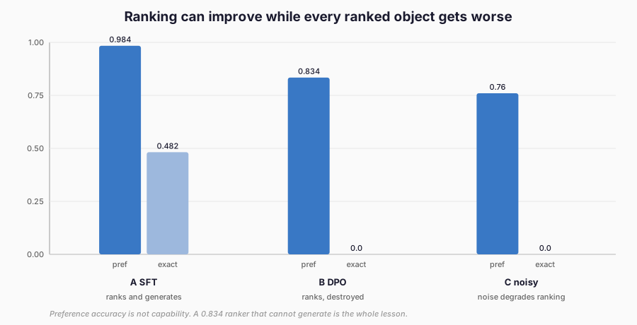
Figure 1. Held-out preference accuracy beside task exact match per arm: SFT achieves preference ranking and correct generation; DPO achieves preference ranking but zero correct greedy completions in the recorded evaluation. Frozen E3 measurements.
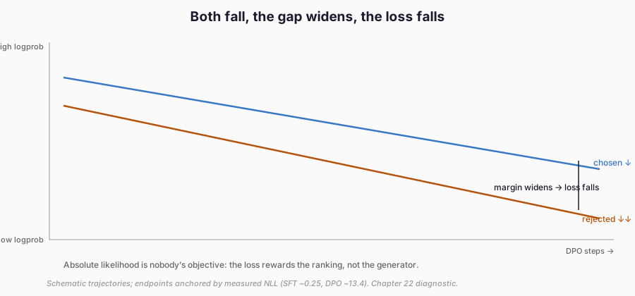
Figure 2. The step-30 diagnostic as motion: both log-probabilities drift down while the margin widens: the preference loss falls as the chosen and rejected log-probabilities decline. In this experimental configuration, the DPO-trained student did not acquire correct generation. Schematic trajectories; endpoints anchored by the measured token NLLs (SFT ~0.25, DPO ~13.4).
On calibration: token-level NLL is reported (A ~0.25, B ~13.4, C ~7.2), but sequence-level calibration of a generator that never formed is not meaningful — confidence over invalid outputs has no decision to inform. The chapter therefore does not claim calibration results beyond the token NLL ledger: where correctness is zero, calibration talk is decoration.
The frozen E3 comparison
Run E3P-20261116T092642Z-8dd412, protocol 1.0 + recording-only
amendment A1, rights RM-114
(train_preference_distillation_e3, verified-permitted, gate
first). Fresh deterministic splits, seeds 20/21/22: train 1200, val
400, test 1000. Teacher w32/L2, 1200 updates, hard CE (val exact
1.0 all seeds; calibration gate passed, not blocking). Frozen SFT
reference = Arm-A best-val checkpoint per seed (hash-audited).
Students w16/L1, EXACTLY 600 updates each, batch 32, Adam 0.002,
identical inits per seed (asserted), best-val restore after the full
budget — A on hard oracle CE, B/C on DPO (β = 0.1) with cached
frozen reference log-probs.
Held-out test pairs for preference accuracy (1000 per seed, built identically from test prompts); greedy decoding for correctness; test ledger appended; no decisions followed from test outcomes. The pair counts mirror the row counts exactly — 1200 train, 400 val, 1000 test — one pair per prompt, so no prompt is ever reused across splits and the preference metric cannot leak training comparisons.
Actual optimiser and token budgets
All 9 students ran exactly 600 updates with identical inits per seed. Target-token exposure: A ~138k, B/C ~277k per seed (chosen plus rejected completions supervised each step — the preference objective sees roughly twice the tokens of SFT for the same update budget; reported, not hidden). Reference forwards: 14 batched forwards per seed for pair caching (1200 train + 400 val pairs × 2 sides, batch 256) plus 1200 counted update-time lookups that cost no forward passes (cached) — caching is seconds of wall time.
Teacher training: w32/L2, 1200 updates, ~43–160 s per seed (host
variable; the work, not the clock, is the budget). Teacher forwards
for dataset generation: zero — pairs are programmatic, no model
calls. Per-arm student wall time across seeds: A 9.4–20.2 s,
B 4.2–10.0 s, C 4.3–10.1 s (B/C validate every 25 steps while A
validates every step under train_fixed_updates; the budget that
matters, updates, matches exactly; the wall-clock difference is host
scheduling plus validation frequency, stated plainly). Total study
wall time 340.8 s, inside the 1800 s ceiling with margin to spare.
Verification cost and failure analysis
Per update: 2 student forwards (chosen + rejected batches) + 0 reference forwards (cached once: 1200 train + 400 val pairs × 2). Teacher training dominates wall time (~43–160 s per seed, host variable) against 9.4–20.2 s per SFT arm and 4.2–10.1 s per DPO arm across seeds — the DPO loop is cheaper per update only because it validates every 25 steps while SFT validates every step; the budget that matters, updates, matches exactly, and the wall-clock gap is disclosed, not hidden.
Pair construction itself costs no model calls (programmatic corruption), and the oracle judge costs nothing beyond the deterministic recomputation — annotation source and cost, as the contract requires: synthetic, free, and auditable, which is also why it cannot stand in for paid human judgement. The failure to analyse is B/C’s, and it is total: exact match 0.000 on every seed, invalid-output rate up to 0.156, reference deviation (mean token KL student||ref on test oracle rows) 25.8/12.3 versus 0.0 for A, token NLL 13.4/7.2 versus 0.25. The equal-size question does not arise (all arms share N = 1200 prompts). The negative result stands as the mission requires: preference optimisation improved the retained ranking signal (0.83/0.76 preference accuracy) while independently measured task correctness was exactly zero at evaluation.
Why DPO is not RLHF, and not SFT either
Three pipelines, different optimised objects. SFT maximises likelihood of demonstrations — no comparisons, no reference. DPO (Eq. 7) minimises classification error on comparisons against a frozen reference — no reward model, no sampling, no policy gradient. RLHF (P-024) fits a reward on comparisons, then optimises it with PPO under a KL constraint — a policy-gradient loop with sampling, baselines, and instability modes DPO was designed to avoid.
Calling DPO “RLHF without the RL” is half true and fully misleading: it shares RLHF’s objective (KL-constrained reward maximisation, per the derivation) and none of its machinery. Calling it “SFT on chosen responses” ignores the rejected term that pushes both likelihoods down here. Our runner computes no policy gradients and samples nothing during DPO training — the test suite pins the frozen reference (no grads, hash-unchanged) and the deterministic pair construction to keep those negatives true.
The contrast the contract asks for, stated concretely: a reward-model pipeline on this task would fit \(r_\phi\) on the same 1,200 pairs (Eq. 2), then run PPO — sampling fresh completions from the student every rollout, scoring them, and updating with a clipped surrogate plus KL penalty. That loop costs orders of magnitude more inference than our cached-reference DPO (zero training-time samples by design) and introduces PPO’s stability knobs. It was not run — deliberately, since the chapter’s question is whether preference distillation says anything beyond direct optimisation, and the honest comparison is SFT-versus-DPO, not DPO-versus-an-unbuilt-RLHF. Do not read the absence as a claim that RLHF would do worse; read it as scope discipline.
Rights, provenance, and limits
Every pair carries prompt, chosen, rejected, pair id, judge id, and
provenance (synthetic-corruption); flipped pairs record the flip.
Arm C’s batch stream used a seed+1 generator (different order than
A/B — disclosed in evidence, not re-run: batch order is not a
claimed control). Nothing is redistributed; no human data exists to
protect, and the rights record says so rather than assuming it.
One design fact bounds the result: the DPO students started from the
same random initialisation as the SFT student, not from the SFT
checkpoint, which served only as the frozen reference.
The experiment therefore tests DPO from scratch against an SFT reference, not DPO applied to an SFT model as its authors recommend. Limitations, without softening: one synthetic instruction task, three seeds, tiny models, oracle judge (not human preference), one corruption type, one β, one noise rate, OOD as longer inputs only, no replication, no independent review. On safety: nothing here transfers. Safety would require human judges, refusal behaviour, adversarial probing, and deployment monitoring — none of which exist in this study, and the chapter claims no safety finding. What the study does contribute to safety thinking is a clean negative example for the safety case of preference methods: a model can satisfy measured preferences perfectly well while being incapable, and any evaluation that reports only the preference metric will miss it.
The strongest caveat is also the most interesting: because even clean DPO failed to produce generation here, this study cannot tell us when preference optimisation preserves correctness — only that ranking can improve while correctness is exactly zero, and that only held-out correctness tells which moved. The obvious next hypotheses are stated, not tested: a larger β (stronger KL anchoring to the reference), an explicit KL penalty term, initialising the DPO policy from the SFT checkpoint, or a reference that already ranks well and generates well might preserve generation while learning rankings. Each is a one-line protocol change and a new experiment — which is exactly where they belong, not in this chapter’s conclusions.
Preparing for continual distillation
Fixed datasets (Chapters 17–19), the student’s own trajectories (Chapter 20), self-generated supervision (Chapter 21), and now comparisons instead of answers (this chapter) — four ways to choose the training signal, and the comparison signal just showed that it can fail to build what the others built. Chapter 23 asks what happens when the signal changes over time: a student that learns task B after task A, with replay, with distillation regularisation, or with nothing — and whether any of it remembers task A.
It inherits the frozen reference (as the pinned old teacher), the fixtures (preference pairs become task-B comparisons), the cost ledger (plus replay storage and teacher-query counts), and the warning: agreement — with a teacher, a judge, or yesterday’s self — is not correctness, and only held-out measurement tells the difference.
References
Rafailov, R., Sharma, A., Mitchell, E., Ermon, S., Manning, C. D. and Finn, C. (2023). Direct Preference Optimization: Your Language Model is Secretly a Reward Model. NeurIPS 2023. https://arxiv.org/abs/2305.18290
Christiano, P. F., Leike, J., Brown, T. B., Martic, M., Legg, S. and Amodei, D. (2017). Deep Reinforcement Learning from Human Preferences. NeurIPS 2017. https://arxiv.org/abs/1706.03741
Ouyang, L., Wu, J., Jiang, X., Almeida, D., Wainwright, C. L., Mishkin, P., Zhang, C., Kaufman, S., Agarwal, S., Slama, K. et al. (2022). Training Language Models to Follow Instructions with Human Feedback. NeurIPS 2022. https://arxiv.org/abs/2203.02155