Ensembles and Multiple Teachers
When several teachers supervise one student, the aggregation rule is the method: probability averaging, logit averaging, and the KL mixture identity behave differently, and the best ensemble is not automatically the best teacher. This chapter derives the identity, measures disagreement, and reports a bounded two-teacher E2 extension.
Two teachers in this chapter’s experiment each classified more than 99% of the test inputs correctly, and they disagreed with each other on only 0.6–1.1% of them. Averaging them added almost nothing: on one seed the average was exactly as accurate as the better teacher. Students trained on that average agreed with it on about 88–89% of inputs, sat about 11 points below its accuracy, and could not be told apart from a student trained on one fixed teacher. Two teachers are not automatically more information than one, and this chapter is about measuring when they are.
Chapter 10 changed the supervision unit from tokens to sequences. This chapter changes the number of supervisors. Instead of one teacher, the student learns from several — and the question is no longer only what to match, but how to combine teachers that are imperfect in different ways.
The central question is:
How should a student combine several imperfect teachers, and when is the best single teacher preferable?
The short answer is that the aggregation rule is the method. Averaging probabilities, averaging logits, and weighting teachers by validation performance are different operations with different guarantees, and none of them turns a better ensemble into a better student automatically. The experiment at the end of this chapter is a deliberately uncomfortable demonstration: two near-perfect, near-identical teachers whose ensemble adds almost nothing, and whose students barely separate.
Why use more than one teacher?
The original motivation for distillation was ensemble compression. Hinton, Vinyals and Dean observe that averaging the predictions of many models is one of the simplest ways to improve almost any learning algorithm, but deploying the whole ensemble is cumbersome; Caruana and collaborators had already shown that the knowledge in an ensemble can be compressed into a single deployable model. The ensemble is the cumbersome model; the student is the deployment model. Everything in this chapter is a special case of that bargain, with the added difficulty that the ensemble members may disagree.
Multiple teachers can help when they are complementary: one teacher is right where another is wrong, and the combination is right more often than either member. But complementarity is a measurement, not a default. Two teachers can also disagree because one of them is simply wrong, or agree so completely that the second teacher adds nothing but cost. This chapter keeps those cases separate by measuring disagreement alongside accuracy at every step.
A preliminary distinction matters. Ensemble distillation (KD-015) transfers supervision from multiple teachers to one student under an explicit aggregation rule. That is different from deploying the ensemble itself (paying the full inference cost forever), from training a student with separate per-teacher objectives without aggregation (a different loss with different gradients), from selecting one teacher per example at deployment (a routing decision, closer to Chapter 28 territory), and from multi-agent or mixture-of-experts systems, where experts specialise and a gate routes each input. Chapter 28 treats those systems; this chapter keeps one student, fixed teachers, and a stated rule for combining them.
Teacher quality and diversity
Before any aggregation, each teacher must be characterised on its own: held-out accuracy, cross-entropy, calibration, error patterns, and inference cost. An ensemble of two 99% teachers behaves nothing like an ensemble of two 70% teachers that err on different inputs, and no weighting rule can be chosen sensibly without those numbers.
Diversity is the gap between “two teachers” and “twice the same teacher”. It can arise from different training seeds, architectures, data, calibration, or inductive biases — but its source does not guarantee its value. Two teachers trained from different seeds on the same data may learn nearly identical functions; two teachers with genuinely different errors may still combine poorly if one of them is miscalibrated and dominates the average. The experiment in this chapter illustrates the first failure deliberately: two same-architecture teachers, different init and shuffle seeds, whose hard predictions disagree on only 0.6–1.1% of test inputs. Their diversity is measurable, real, and almost entirely useless.
That negative framing is the point. A chapter that only shows complementary teachers would teach the reader that ensembles help; a chapter that also shows correlated teachers teaches the reader when they do not.
Probability averaging
Suppose there are \(M\) teachers producing distributions \(p_1(y\mid x),\ldots,p_M(y\mid x)\) over the same classes in the same order. Choose non-negative weights summing to one, \(w_j\ge0\), \(\sum_jw_j=1\), and define the ensemble distribution
\[ \bar p(y\mid x)=\sum_jw_jp_j(y\mid x). \]
Because each \(p_j\) is non-negative and sums to one, so is \(\bar p\): non-negativity is inherited term by term, and normalisation follows from linearity of summation. Uniform averaging sets \(w_j=1/M\); weighted averaging tilts toward teachers trusted more. When one teacher receives all the weight, the ensemble reduces to that teacher. When teachers agree, every reasonable average reproduces their shared distribution. When they strongly disagree, the mixture sits between them — which is a compromise, not a resolution. A mixture of a correct confident teacher and a wrong confident teacher can be confidently wrong about both, or weakly right; the arithmetic does not know which.
Example A. Two teachers over three classes: \(p_1=[0.7,0.2,0.1]\), \(p_2=[0.4,0.4,0.2]\). The uniform mixture is \([0.55,0.30,0.15]\): teacher 1 predicts class 1, teacher 2 predicts class 1, the ensemble predicts class 1 — agreement all the way down, and the mixture conceals how differently confident the teachers were. With weights \((0.75,0.25)\) the mixture is \([0.625,0.25,0.125]\). Move the weight to \((1,0)\) and the ensemble is exactly teacher 1; the endpoint recovers the single-teacher case, which is why “best single teacher” is always a legitimate competitor to any average.
Logit averaging
Let teacher logits be \(z_1,\ldots,z_M\) and define the weighted logit aggregate \(\bar z=\sum_jw_jz_j\), then \(\mathrm{softmax}(\bar z/T)\). This generally differs from averaging the probability distributions, \(\sum_jw_j\mathrm{softmax}(z_j/T)\). The two operations commute only in special cases; in general, averaging before the nonlinearity is not averaging after it.
There is a precise relationship worth stating. Exponentiating the averaged logits gives \(\exp(\bar z_i/T)=\prod_j\exp(z_{ji}/T)^{w_j}\), a weighted geometric mean of the teachers’ unnormalised exponentials. After normalisation, logit averaging is a normalised geometric mean of the teachers’ scaled exponentials — whereas probability averaging is an arithmetic mean of normalised distributions. Geometric means punish disagreement more harshly: one teacher assigning near-zero probability to a class nearly vetoes it under logit averaging, while arithmetic averaging lets the other teachers outvote.
Example A continued. With \(z_1=[2,1,0]\) and \(z_2=[1,1,1]\): \(\mathrm{softmax}(z_1)=[0.6652,0.2447,0.0900]\), \(\mathrm{softmax}(z_2)=[1/3,1/3,1/3]\), and the uniform probability mixture is \([0.4993,0.2890,0.2117]\). Logit averaging gives \(\bar z=[1.5,1.0,0.5]\) and \(\mathrm{softmax}(\bar z)=[0.5065,0.3072,0.1863]\). Same teachers, same weights, different ensemble — class prediction agrees here, but the distributions differ in every entry. A reader who treats the two averages as interchangeable will misreport what the student was actually trained on.
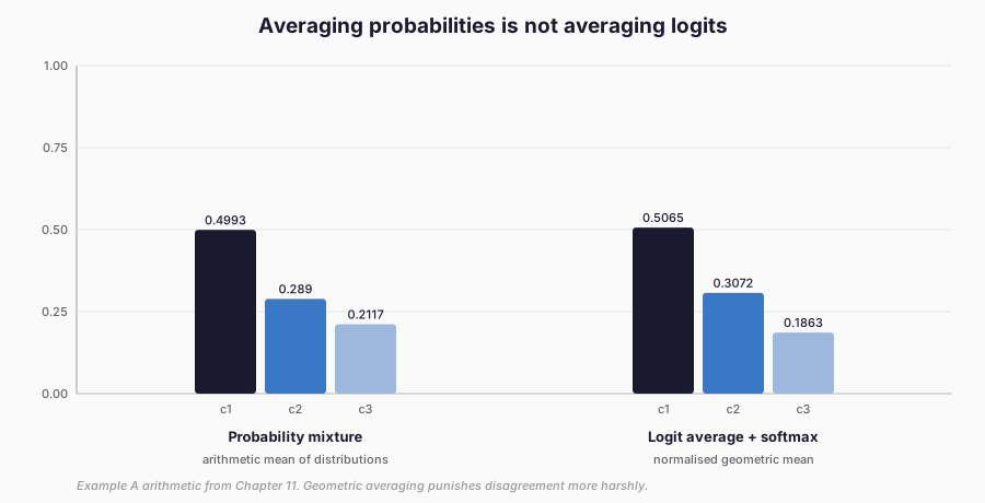
Figure 1. Example A drawn twice: the uniform probability mixture against the softmax of the averaged logits. Same teachers, same weights, different targets — arithmetic mean against normalised geometric mean. Worked arithmetic, not measured data.
Two compatibility warnings follow. First, logit scales must be comparable: logits from models trained at different temperatures, with different regularisation, or with different output biases live on different scales, and their average is not meaningful without recalibration. Second, softmax is offset-invariant (adding a constant to all logits of one teacher leaves its distribution unchanged), so two teachers can have wildly different raw logits and identical distributions — or identical-looking logits and different effective temperatures. The implementation tests offset invariance explicitly: shifting one teacher’s logits by a constant changes the logit average’s raw values but the probability mixture is untouched. Arbitrary scores from incompatible models must never be averaged; the compatibility check in this chapter rejects permuted class orders and mismatched tokenisers even when the tensor shapes match.
Because of these differences, this chapter’s experiment uses probability averaging only. Logit averaging is derived, unit-tested as a counterexample, and left out of the training comparison — a deliberate boundary, not an oversight.
The multi-teacher KL identity
This is the chapter’s central mathematical result. For fixed teacher distributions \(p_j\), student distribution \(q\), and weights \(w_j\), let \(\bar p=\sum_jw_jp_j\). Then
\[ \sum_jw_jD_{\mathrm{KL}}(p_j\parallel q) =D_{\mathrm{KL}}(\bar p\parallel q) +\sum_jw_jD_{\mathrm{KL}}(p_j\parallel\bar p). \]
The proof is one expansion. Write each KL as an expectation under \(p_j\), collect terms, and add and subtract \(\log\bar p\):
\[ \begin{aligned} \sum_jw_j\sum_yp_j(y)\log\frac{p_j(y)}{q(y)} &=\sum_jw_j\sum_yp_j(y) \left[\log\frac{p_j(y)}{\bar p(y)}+\log\frac{\bar p(y)}{q(y)}\right] \\ &=\sum_jw_jD_{\mathrm{KL}}(p_j\parallel\bar p) +\sum_y\left(\sum_jw_jp_j(y)\right)\log\frac{\bar p(y)}{q(y)} \\ &=\sum_jw_jD_{\mathrm{KL}}(p_j\parallel\bar p) +D_{\mathrm{KL}}(\bar p\parallel q). \end{aligned} \]
The final term is the weighted Jensen–Shannon disagreement among the teachers: it measures how far each teacher sits from the consensus, and it contains no \(q\). For fixed teachers and fixed weights, the disagreement term is a constant of the optimisation — the two objectives on either side have identical student gradients and identical minimisers, subject to the same optimisation constraints. Their loss values differ by exactly that constant, so loss values across the two formulations must never be compared directly.
The assumptions matter and are stated plainly. All distributions share the same support over the same classes in the same order; where a probability is zero, the convention \(0\log0=0\) applies and the implementation clamps tiny probabilities for numerical safety. The equivalence covers forward KL from an arithmetic probability mixture only. It does not apply to reverse KL, to raw-logit MSE, to nonlinear aggregation such as logit averaging followed by softmax, to incompatible output spaces, or to student-dependent weights — if the weights depend on \(q\), the disagreement term moves with the student and the gradients differ. An adaptive weighting method that makes weights a function of the student’s state is therefore a different objective, not a free application of the identity.
Example B. With the Example A distributions and student \(q=[0.5,0.3,0.2]\): \(D_{\mathrm{KL}}(p_1\parallel\bar p)=0.047174\), \(D_{\mathrm{KL}}(p_2\parallel\bar p)=0.045228\), disagreement \(=0.046201\); \(D_{\mathrm{KL}}(\bar p\parallel q)=0.009268\); weighted teacher KL \(=0.055469\); and \(0.009268+0.046201=0.055469\). The implementation’s test verifies the same identity on random distributions and additionally checks that student gradients under both formulations agree to \(10^{-5}\) — the formulation changes the loss value, not the update.
Teacher disagreement
Disagreement needs several measures because no single number separates “useful diversity” from “one teacher is wrong”. This chapter records, per teacher pair: hard-label disagreement rate; mean pairwise L1 distance (halved, so identical to total variation on two distributions); the Jensen–Shannon disagreement at deployment temperature; ensemble accuracy; and the correctness-pattern rates — both correct, exactly one correct, both wrong. The last three are the diagnostic core: an ensemble can only help on the “exactly one correct” slice (where the combination might pick the right member) and is helpless on the “both wrong” slice.
In the E2 extension, the pattern table is sobering. Both teachers are correct on 98.9–99.3% of test inputs; exactly one is correct on 0.5–1.0%; both are wrong on 0.1–0.4%. The ensemble’s accuracy gain over its members is 0.1–0.3 percentage points. There is almost no “exactly one correct” slice to exploit, so even a perfect aggregation rule has nothing to work with.
High disagreement would not have fixed this either: had the teachers disagreed widely with one of them wrong, the mixture would sit between right and wrong without knowing which is which. Disagreement is information about the teachers, not evidence that combining them helps.
Du et al. (2020) frame this conflict in gradient space and propose regarding ensemble distillation as multi-objective optimisation with a tolerance parameter — a dynamic per-teacher weighting view. That direction is cited here for the disagreement concept only. Its exact gradient-space algorithm is not reproduced, and this chapter’s experiment implements only static validation weights: the honest, checkable subset of the idea that fits the compute budget and the frozen protocol.
Choosing and weighting teachers
Five policies cover the practical space:
- Uniform ensemble. Every teacher receives equal weight. No selection, no fitting, no failure mode beyond the compromise itself.
- Validation-weighted ensemble. Weights are fixed globally from a predeclared validation metric — here, inverse validation cross-entropy, clamped to \([0.1,0.9]\) and renormalised. Computed on validation data only, frozen before training.
- Best single teacher. The teacher with the lower validation CE; exact ties select teacher A. A legitimate competitor, not a straw man.
- Fixed single teacher. A rotation fixed before the run (seeds 0→A, 1→B, 2→A): reproducible, metric-independent, and independent of held-out test outcomes. It separates “a single teacher” from “the selected teacher”.
- Disagreement-aware weighting. The Du et al. direction: weights that respond to conflict. Discussed, not trained here — its behaviour and cost could not be validated inside this chapter’s scope, and an unvalidated adaptive method would be decoration.
Two prohibitions are load-bearing. Never fit weights on test labels. Never use per-example oracle weighting that peeks at ground truth unavailable at deployment. Both would manufacture an advantage the deployed system cannot reproduce.
When teachers conflict
Conflict has three shapes. Correlated error (both wrong together) is immune to averaging: the mixture of two identical wrong distributions is wrong. One-sided error (exactly one correct) is exploitable only if the aggregation favours the right member without knowing the label — validation weights can do this on average, not per example. Calibration conflict occurs when a wrong but overconfident teacher dominates a right but diffuse one; temperature scaling and validation weighting mitigate it, but neither resolves it per example.
Stanton et al. (2021) add the deeper caution: even when the student has capacity to match the teacher, a fidelity gap typically remains, optimisation difficulty is a key cause, and closer fidelity does not always improve generalisation. For ensembles this cuts twice. First, matching the mixture is harder than matching one teacher, so the student–ensemble gap can exceed the single-teacher gaps. Second, even perfect mixture fidelity would only reproduce the ensemble’s accuracy — which, when teachers are near-identical, barely exceeds the members. The experiment below shows both effects in miniature: students agree with the ensemble on ~88% of inputs yet sit ~11 points below its accuracy.
Output-space compatibility
Aggregation is only defined when teachers speak the same output language. Before any averaging, the implementation requires: same task, same class semantics, same class ordering, same class count (or an explicit valid mapping), compatible temperature treatment, and finite, well-shaped tensors. For language models the same rule applies to token identities, not tensor lengths: two models with different tokenisers cannot have their probability vectors averaged just because the vectors happen to be equally long.
Example C. Two teachers output 4-dimensional distributions over \([a,b,c,d]\), but the second teacher was trained with order \([b,a,c,d]\). Shapes match; semantics do not. Averaging entry-wise mixes \(p(a)\) with \(p(b)\) and produces a distribution over nothing. The compatibility check rejects the pair before any number is computed — and the test suite verifies rejection for permuted orders, mismatched tokeniser ids, and mismatched class counts. No automatic tokeniser-alignment mechanism is invented; at this budget, rejection is the correct behaviour.
The controlled experiment
The E2 four-class shape task is reused unchanged (1,200/400/1,000 splits,
noise 0.25, seeds 0–2). Two teachers share the E2 teacher architecture
(channels \([16,32]\), 4,932 parameters) and data partition, differing
only in init/shuffle seed (A: seed, B: seed+5000). The student keeps the
E2 student architecture (\([4,8]\), 372 parameters). All arms use the
E2-style objective — hard CE plus \(0.5\cdot T^2\)KL at \(T=2\) — with
only the target varying:
| Arm | Student supervision |
|---|---|
| A-hard | Ground-truth labels only |
| B-best-single | Best-validation teacher |
| C-uniform | Uniform \((0.5,0.5)\) mixture |
| D-weighted | Validation inverse-CE mixture, clamped, frozen |
| E-fixed-single | Rotation teacher (0→A, 1→B, 2→A) |
Forty epochs, patience 8, Adam, batch 64, ground-truth validation CE for
every arm — the same rule E2 used, so arm A reproduces the historical E2
baseline per seed (0.790/0.873/0.969) exactly. No projector: all arms are
output-level, isolating the aggregation rule. Rights record RM-105 covers
only train_and_evaluate_e2_ensemble; the run completed in 91.2 s on CPU
(teacher training 19.4 s), inside the 30-minute ceiling.
Student accuracy versus ensemble accuracy
Teachers are near-perfect and near-identical: A scores 0.9950/0.9940/0.9940, B scores 0.9930/0.9970/0.9910, and the uniform ensemble reaches 0.9960/0.9970/0.9950. Hard disagreement is 0.6–1.1%; JS disagreement is 0.006–0.008. Validation weights come out (0.61,0.39), (0.56,0.44), (0.51,0.49) — the third pair is uniform for all practical purposes, and seed 2’s D arm indeed equals C to four decimals.
| Arm | Accuracy (%) | CE | ECE | Probe (%) |
|---|---|---|---|---|
| A-hard | 87.73 ± 8.96 | 0.36 ± 0.22 | 0.10 ± 0.04 | 86.37 ± 9.04 |
| B-best-single | 88.37 ± 7.28 | 0.31 ± 0.18 | 0.06 ± 0.03 | 85.47 ± 8.26 |
| C-uniform | 88.40 ± 7.91 | 0.32 ± 0.19 | 0.07 ± 0.02 | 85.57 ± 7.70 |
| D-weighted | 88.20 ± 7.96 | 0.32 ± 0.19 | 0.07 ± 0.02 | 85.33 ± 7.75 |
| E-fixed-single | 88.40 ± 7.27 | 0.31 ± 0.18 | 0.07 ± 0.03 | 85.57 ± 8.32 |
Per seed, accuracy reads: seed 0 — 0.790/0.820/0.811/0.811/0.820; seed 1 — 0.873/0.868/0.873/0.867/0.869; seed 2 — 0.969/0.963/0.968/0.968/0.963. Three patterns deserve emphasis, and none supports a universal ranking.
First, every distillation arm beats the baseline on seed 0 (+2–3 pp). On seed 1, arm C ties the baseline exactly and the other arms fall below it; on seed 2 the baseline wins outright. The mean differences (+0.47 to +0.67 pp) are dwarfed by the seed spread (7–9 pp). This is a null-to-small result, reported as such.
Second, C, D, and E are indistinguishable (88.20–88.40%). With teachers this correlated, the weighting rule has nothing to grip: uniform, validated, and single-teacher targets carry nearly the same information, and the students learn nearly the same function. Student–ensemble agreement sits at ~88–89% for every arm — the students imitate the ensemble about equally, and all fall ~11 points short of its 99.5%+ accuracy, exactly the fidelity gap Stanton et al. describe.
Third, calibration and likelihood favour the distillation arms (CE 0.31–0.32 vs 0.36, ECE 0.06–0.07 vs 0.10) while the linear probe slightly favours the baseline (86.37% vs 85.33–85.57%) — the same qualified pattern E2 reported for its feature arms. No arm dominates on every metric, so no arm is declared the winner.
Teacher and deployment cost
Two teachers double the expensive parts: teacher training cost 19.4 s total (two full training runs), and teacher inference costs two forward evaluations per input (2,000 evaluations per 1,000-input pass). Student training takes 1.6 s (hard) to 4.6 s (two-teacher arms — the extra teacher forward pass per batch is visible). Deployment costs one 372-parameter student in every arm (1,488-byte artefact scale), against 9,864 parameters to serve both teachers plus the averaging logic.
The student is attractive not because it beats the ensemble — it does not, losing ~11 points — but because it recovers the baseline-or-better accuracy at one model’s cost with better calibration. When the ensemble’s edge is large and its cost affordable, serving the ensemble is the honest recommendation; distillation is for when deployment, not accuracy, is the constraint.
Rights and provenance
Every teacher in an ensemble carries its own rights status, and the combination inherits the strictest constraint: averaging outputs does not launder their restrictions. This extension sidesteps the hard case by construction — both teachers are self-created under RM-105, same task, same licence, no external sources — but the workflow does not. The manifest records each teacher’s architecture, training seed, checkpoint identity, validation and held-out metrics, error overlap, and evaluation cost; the aggregation rule, weights, and weight-selection inputs are frozen in the protocol and config. A future ensemble mixing external teachers would need each source’s terms checked separately (storage, training use, redistribution, competing-model clauses) before any averaging, because an ensemble output encumbers the student with every source’s restrictions at once. Chapters 36–39 develop that analysis; no rights record was changed in this stage.
When one teacher is better
One teacher wins outright when teachers are near-identical (this experiment), when the weaker teacher is wrong more often than complementary, when validation data is too thin to estimate weights reliably (uniform then dominates by default), when calibration conflict lets a confident wrong teacher dominate the mixture, and when the teacher-query budget forbids consulting two models per input.
The engineering default should be: train the hard baseline (arm A), distil from the best validation teacher (arm B), and add the uniform ensemble (arm C) only if disagreement diagnostics show a usable “exactly one correct” slice. Validation weighting (arm D) earns its place when teachers differ stably in quality; here it reproduces C, which is itself a finding about these teachers.
    flowchart TD
  A[train hard baseline] --> B[distil from best-validation teacher]
  B --> D{usable 'exactly one correct' slice?}
  D -->|yes| C[add uniform ensemble]
  D -->|no| S[stop: one teacher is enough]
  C --> W{teachers differ stably in quality?}
  W -->|yes| V[try validation weighting]
  W -->|no| S
Figure 2. The selection order the experiment justifies: each stage must earn its place against the previous one.
Limits of this chapter’s evidence
- Set-up: two self-created teachers that share an architecture and a data partition and differ only in their initialisation and shuffle seeds, on one synthetic shape task. This is the correlated-teacher case by design; no complementary teachers were tested.
- Measurements: three seeds. The mean differences between arms (+0.47 to +0.67 points) are far smaller than the 7–9 point spread between seeds and do not support a ranking. Timings are local CPU measurements.
- Implementation: probability averaging only, with static validation weights. Logit averaging and disagreement-aware weighting are derived or discussed, not trained.
- Scope: Examples A–C are worked arithmetic. The Du et al. and Stanton et al. findings are their authors’ reports and were not reproduced. Nothing here shows when ensembles of genuinely different teachers help a student.
What Part II has established
Part II — Classical Distillation — is now drafted in full. Its arc runs from outputs (Chapter 06: probabilities, logits, rankings, DKD), through access regimes (Chapter 07: top-k, samples, query economics), targets (Chapter 08: features and projections; Chapter 09: attention and relations), sequences (Chapter 10: beam targets, length and exposure bias), to teachers themselves (this chapter: aggregation, disagreement, selection). Three lessons recur and are worth stating once. First, the objective defines what is optimised: matching distributions, values, relations, sequences, or mixtures are different claims with different gradients. Second, agreement is not correctness: teacher–student, student–ensemble, and teacher-forced metrics diagnose imitation, never substitute for held-out task performance. Third, cost is part of the method: query budgets, beam-search bills, and teacher counts belong in the protocol, not in a footnote. The E1, E2, and E3-precursor programmes leave open the data question — what the transfer set contains, how it is chosen, and what may lawfully go into it. That is Part III’s subject, beginning with Chapter 12, The Data Behind the Knowledge.
References
Hinton, G., Vinyals, O. and Dean, J. (2015). Distilling the Knowledge in a Neural Network. NIPS 2014 Deep Learning Workshop. arXiv:1503.02531. https://arxiv.org/abs/1503.02531
Du, S., You, S., Li, X., Wu, J., Wang, F., Qian, C. and Zhang, C. (2020). Agree to Disagree: Adaptive Ensemble Knowledge Distillation in Gradient Space. Advances in Neural Information Processing Systems 33. https://papers.nips.cc/paper/2020/hash/91c77393975889bd08f301c9e13a44b7-Abstract.html
Stanton, S., Izmailov, P., Kirichenko, P., Alemi, A. A. and Wilson, A. G. (2021). Does Knowledge Distillation Really Work? Advances in Neural Information Processing Systems 34. https://papers.neurips.cc/paper_files/paper/2021/hash/376c6b9ff3bedbbea56751a84fffc10c-Abstract.html