Feature-Based Distillation
Intermediate representations can carry structure that final outputs discard, but feature matching requires a projection, a layer correspondence, and a separate test of task correctness. This chapter derives feature MSE and cosine losses and reports the bounded E2 experiment.
Two students in this chapter’s experiment were trained to imitate the same teacher layer in different ways. One matched the layer’s values; the other matched only their directions. Their cosine distances from the teacher ended up almost identical, 0.077 and 0.079, while their feature errors were 0.318 and 1.279. Both had slightly higher mean accuracy than a student trained on labels alone, but by less than the 7–9 point spread between seeds. Looking more like the teacher inside the network and doing better on the task are separate outcomes, and this chapter measures them separately.
Chapter 07 treated the teacher’s output interface as the constraint. A top-1 label, a top-k list, or a sampled class exposes only part of the teacher’s final prediction. This chapter moves inside the network. The teacher’s intermediate representation may contain structure that never survives the final softmax: edges, textures, parts, spatial arrangements, or task-specific features.
The central question is:
Does matching a teacher’s internal representation provide useful information that matching its outputs cannot, and what does that additional access cost?
The answer is not automatic. Features are high-dimensional, architecture specific, and often unavailable. A student can be made to look more like its teacher in a hidden layer without becoming more correct on the task. Feature similarity is a diagnostic, not the headline result.
The signal inside the network
An intermediate representation is a tensor produced by a hidden layer. In a
convolutional network it is usually a feature map with shape
[batch, channels, height, width]. In a transformer it is a sequence of hidden
states with shape [batch, tokens, features]. In an embedding model it may be a
single vector per input.
These tensors are not interchangeable with logits. A logit is a score for one class. A feature map is a learned description of the input at a particular depth. It can encode information that the final classifier uses, but it can also encode information the classifier ignores. It may be sensitive to position, texture, contrast, or batch statistics. It may change meaning between architectures.
A convolutional feature map has three axes: batch, channel, and spatial position. A channel may respond to an oriented edge, a colour transition, or a texture; a spatial position records where that response occurred. Later layers often have larger receptive fields and more semantic responses, but the mapping from channel to concept is learned, not declared. A transformer hidden state has batch, token, and feature axes; its meaning depends on the tokeniser, position encoding, and layer. Nothing in the tensor shape says which coordinates should correspond across two models.
Feature distillation (KD-012) is training a student with supervision from a teacher’s intermediate representation. Representation alignment (KD-029) is the construction of a meaningful comparison between the teacher and student feature spaces. The two concepts belong together: a feature loss without a defensible alignment is a comparison of unrelated tensors.
The feature-mismatch problem
Let the teacher’s hidden representation be
A trainable projection supplies a bridge:
A projection that makes two tensors the same shape does not make their contents semantically equivalent. It creates a differentiable comparison, not a correspondence. The choice of layer pair and projection is a modelling decision, and it has to be evaluated like any other modelling decision.
A fixed projection is appropriate when the correspondence is known and simple: for example, a channel permutation or a shared spatial grid. A learned projection is necessary when the student’s channel organisation differs from the teacher’s, as it usually does. The learned projector can absorb some of that mismatch, but it adds parameters and can overfit a small training set. The projector’s cost belongs to training, not deployment, but it is still part of the experiment’s parameter budget.
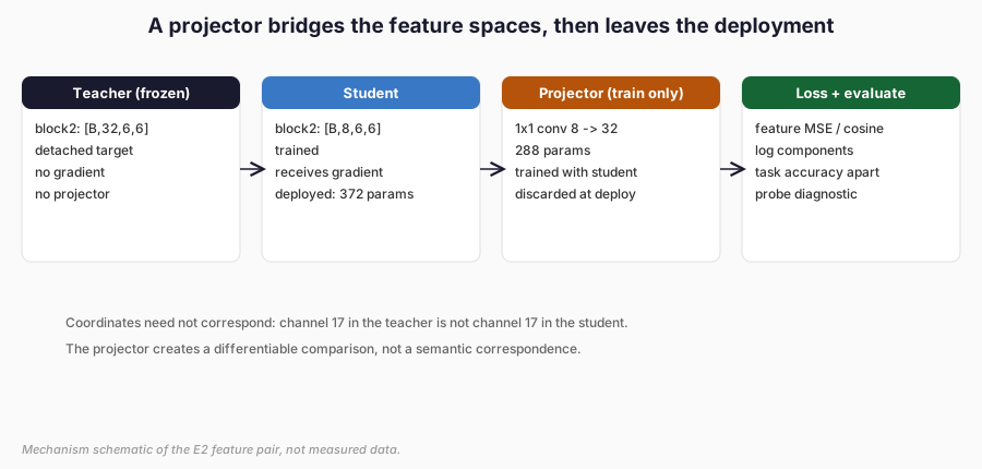
Figure 1. The E2 feature pair as a training system. The frozen teacher supplies the target; the student and the 288-parameter projector learn; the projector is discarded before deployment. Mechanism schematic, not measured data.
A compact CNN alignment using the tested interface is:
teacher_out = teacher.forward_with_features(images)
student_out = student.forward_with_features(images)
projector = FeatureProjector(8, 32, kind="conv")
aligned = projector(student_out.features["block2"])
loss = feature_mse(aligned, teacher_out.features["block2"].detach())
For a transformer-style check, let teacher hidden states have shape
[2, 5, 64] and student hidden states [2, 5, 24]. A linear projector
24 -> 64 gives [2, 5, 64]; feature MSE and cosine use dim=-1. The tests
verify this shape alignment. No transformer model is trained for the example.
Projection and alignment design
For convolutional feature maps, a 1x1 convolution is a natural projector when the spatial sizes match. It mixes channels without changing the spatial grid. For vector or transformer hidden states, a linear map on the final dimension is the usual choice.
In E2, the teacher’s second block produces [batch, 32, 6, 6]; the student’s
second block produces [batch, 8, 6, 6]. A 1x1 convolution maps 8 channels to
32 and preserves the 6x6 grid. It has
If the spatial resolutions differ, there are three honest options: choose a different layer pair, use a justified spatial alignment, or reject the pair. Silent interpolation or reshaping changes the meaning of the comparison. The implementation checks shapes and raises an error rather than guessing.
Feature MSE
For aligned features of dimension \(d\), the per-example feature MSE is
The gradient with respect to the aligned student feature is
A small hand calculation makes the scale visible. Take
The reduction convention matters for feature maps. A mean over every channel, row, and column gives each spatial position and channel equal weight. A sum scales with the size of the map. A per-position mean followed by a batch mean changes the balance between positions and examples. The implementation must state the convention, and the coefficient must be interpreted against that convention. E2 uses a mean over all feature elements, then a batch mean.
Feature magnitude matters. A feature loss with a large numerical scale can dominate the task cross-entropy even when its coefficient looks small. The coefficient is part of the objective, and the loss components should be logged separately during training.
Cosine feature matching
Cosine matching compares directions rather than coordinates:
For a single vector, the gradient with respect to the aligned student feature is
Cosine and MSE preserve different things. Positive rescaling preserves cosine but changes MSE. Translation generally changes cosine and MSE. For \(\hat h_S=(1,0)\) and \(h_T=(1,1)\), the cosine loss is \(1-1/\sqrt2\approx0.293\). Rescaling the student to \((2,0)\) leaves the loss unchanged; translating it to \((2,1)\) changes the loss. Cosine is useful when direction is the intended signal. It is not a drop-in replacement for MSE.
The tests check the formulas against autograd, verify positive-scale
invariance, and verify that translation is not invariant. For feature maps, the
same formula is applied at each spatial position with dim=1; for transformer
states, it is applied at each token with dim=-1. The dimension is an explicit
argument, not an implementation detail that changes silently.
Normalisation and spatial semantics
Feature matching often needs a normalisation decision:
- L2 normalisation compares direction and removes magnitude.
- Mean centring removes a common offset.
- Channel standardisation puts channels on a comparable scale.
- Learned projection lets the model choose the mixing.
- Fixed projection imposes a correspondence chosen by the engineer.
Each choice discards something. L2 normalisation discards magnitude; centring discards a common offset; channel standardisation discards per-channel scale and shift. A learned projection can recover some of that information, but it adds parameters and can overfit.
The same class decision can arise from differently organised hidden representations. One network may put evidence for a shape in channel 3, another in channels 7 and 9. Matching a single layer assumes a correspondence that the architectures did not necessarily learn. That is why a projection is necessary and why a successful projection does not prove that the teacher’s representation is the unique correct target.
Channel standardisation needs particular care. If the mean and standard deviation are computed from the current batch, the target changes with batch composition and can leak information across examples. If they are computed from the training set, the statistics must be frozen before evaluation. Either way, the choice belongs in the protocol, not in an undocumented helper.
FitNets: hints and staged training
Romero et al. (2015) introduced hints for thin and deep students. A teacher hint layer supervises a student guided layer through a regressor. The hint loss is
The original procedure has two stages. The first trains the student up to the guided layer and the regressor against the hint. The second trains the whole student with the knowledge-distillation objective, starting from the guided parameters. For convolutional maps, the paper uses a convolutional regressor rather than a huge fully connected one, so the number of parameters stays manageable. The staging matters: it gives the student a representation-level initialisation before the output objective is applied.
Our E2 implementation is not a FitNets replication. It uses a single-stage combined objective:
Contrastive representation distillation
Tian et al. (2020) argue that output KL ignores structural knowledge in the teacher representation. Their contrastive objective trains the student to capture relationships among examples and representations, not only pointwise feature values. The abstract reports gains over knowledge distillation and other distillers on several transfer tasks. Those results are external and were not replicated here.
Contrastive representation distillation is introduced as a direction, not implemented in E2. Chapter 09 develops relational objectives. Adding a contrastive loss here would require a different experiment, negative sampling, and a separate evaluation; it is not a free extension of pointwise feature MSE.
The distinction is structural. Pointwise MSE treats each feature coordinate as an independent target. Contrastive methods compare examples and can preserve similarity relationships that coordinate-wise matching may miss. A method can combine both signals, but the combination needs its own ablation and budget.
The E2 experiment
E2 asks whether feature supervision improves held-out task performance at a matched student architecture and budget. The data are synthetic 12x12 grayscale images with four shape classes: horizontal bar, vertical bar, down-right diagonal, and down-left diagonal. Position and Gaussian noise vary independently of the label. The splits are 1,200 train, 400 validation, and 1,000 test, with noise 0.25.
The teacher is a convolutional classifier with channels (16, 32), 4,932
parameters. The student uses the same architecture family with channels
(4, 8), 372 parameters.
Layer selection in E2
The chosen pair is the second block. The first block is an unmeasured candidate, and a flattened linear projection is listed to show why the 1x1 convolution was preferred.
| Pair | Teacher shape | Student shape | Projection | Training params | Measured |
|---|---|---|---|---|---|
| Block 1 | 16 x 12 x 12 | 4 x 12 x 12 | 1x1 conv, 4 -> 16 | 80 | No |
| Block 2 (chosen) | 32 x 6 x 6 | 8 x 6 x 6 | 1x1 conv, 8 -> 32 | 288 | Yes |
| Block 2 linear | 32 x 6 x 6 | 8 x 6 x 6 | flattened linear, 288 -> 1,152 | 332,928 | No |
Block 2 gives a deeper, more semantic representation and a modest projector. The flattened linear alternative has more than three hundred thousand training parameters for a 372-parameter student; it was rejected on cost before the run. Block 1 was not measured. No test data was used to choose the pair.
The feature pair is teacher [batch, 32, 6, 6] and student
[batch, 8, 6, 6], projected by a 1x1 convolution 8 -> 32 with 288
training-only parameters.
| Arm | Objective |
|---|---|
| A-hard | Ground-truth cross-entropy |
| B-output-kl | CE + 0.5 * \(T^2 D_{\mathrm{KL}}(p_T^{(T)}\parallel p_S^{(T)})\), \(T=2\) |
| C-feature-mse | CE + 0.5 * projected feature MSE |
| D-feature-cosine | CE + 0.5 * projected feature cosine |
All arms use the same student, optimiser, 40-epoch cap, validation cross-entropy for checkpoint selection, and one held-out test evaluation. Feature coefficients were fixed before the run; no coefficient or layer sweep was performed. The teacher is frozen; its features are detached.
The teacher reached 99.4-99.5% test accuracy across three seeds. The student results were:
| Arm | Accuracy (%) | CE | ECE | Agreement (%) | Probe (%) |
|---|---|---|---|---|---|
| A-hard | 87.73 ± 8.96 | 0.3604 ± 0.2223 | 0.1016 ± 0.0358 | 87.57 ± 9.06 | 86.07 ± 9.27 |
| B-output-kl | 88.37 ± 7.28 | 0.3132 ± 0.1841 | 0.0650 ± 0.0307 | 88.33 ± 7.48 | 85.57 ± 8.32 |
| C-feature-mse | 89.07 ± 8.32 | 0.3864 ± 0.1846 | 0.1436 ± 0.0211 | 89.07 ± 8.52 | 86.70 ± 9.53 |
| D-feature-cosine | 88.73 ± 7.90 | 0.3682 ± 0.2200 | 0.1240 ± 0.0469 | 88.73 ± 8.05 | 86.53 ± 9.39 |
The feature arms have slightly higher mean accuracy than the baseline: C by 1.33 percentage points and D by 1.00. B is 0.63 points above A. But the seed spread is 7-9 percentage points. The differences are descriptive, not significant. The feature arms do not show a consistent cross-entropy or calibration advantage: C and D have higher CE and ECE than A, while B has the lowest CE and ECE. The linear probe is also nearly flat: 85.6-86.7% across arms, within the seed spread.
The representation diagnostics are more specific. C’s projected feature MSE is 0.318 and its cosine distance is 0.077. D’s MSE is 1.279 and its cosine distance is 0.079. D’s cosine objective matches direction about as well as C, but with a much larger magnitude error. That is a useful illustration: cosine and MSE are different objectives, not two names for the same similarity. Neither diagnostic guarantees a task improvement.
The experiment is therefore a qualified null-to-small-positive result. Feature supervision did not produce a clear, consistent task advantage on this task and budget. It also did not produce a clear representation advantage on the linear probe. The correct conclusion is not “feature distillation fails”; it is that this particular layer pair, projection, coefficient, task, and budget did not demonstrate a reliable gain.
E2 did not test staged FitNets training, other layer pairs, other projection types, a coefficient sweep, or contrastive objectives. Those are separate experiments, not missing cells in this one. The unmeasured candidates in the layer table are labelled as unmeasured for that reason.
Linear probes
A linear probe asks whether the student’s frozen representation contains
information that a simple classifier can use. After training, the student’s
native block2 feature map is global-average-pooled to an 8-dimensional vector.
A linear classifier is trained on the 1,200 training features, selected on the
400 validation features, and evaluated once on the 1,000 test features. The probe
has 36 parameters and does not update the student.
Probe accuracy is informative but incomplete. It measures linear separability, not the full utility of the representation. A representation can be useful for a nonlinear head while a linear probe underperforms. A probe can also overfit the training features. The probe is a diagnostic, not a substitute for held-out task accuracy.
The probe budget is separate from the student budget. E2 used at most 100 epochs, patience 10, and a 36-parameter linear classifier. The probe never updated the student, and the test features were read once. A larger probe or a nonlinear head could produce a different ranking; that would be a different diagnostic, not a correction of the student result.
Costs and rights
The student has 372 parameters and a 1,488-byte state dict. The projector has 288 training-only parameters; it is excluded from deployment. Mean student training time was 3.02 s for A, 5.64 s for B, 6.91 s for C, and 8.29 s for D. Median latency was about 0.73-0.75 ms per measured batch in this environment. Peak process memory was 526.5 MB cumulative high-water mark. These are local measurements, not deployment benchmarks.
Feature access is also an interface question. Some services expose embeddings but not hidden maps; some expose a final hidden state but not an intermediate layer; some expose nothing beyond text. A layer can be inaccessible even when the model is otherwise open. The experiment must record the exact layer, the tensor shape, and whether the teacher-side computation is available at training time.
Feature access is a rights question. Intermediate activations are model-derived
outputs. They can carry information about inputs, training data, or internal
representations, and they may be subject to confidentiality, personal-data, or
contractual constraints. A black-box API generally does not expose intermediate
features; a local open-weight teacher may, but the licence still governs the
permitted action. E2 used only self-created images and models under RM-103,
which authorises train_and_evaluate_e2. It did not use external data,
pretrained weights, or a provider API. The record was separate from RM-101 and
RM-102 and did not broaden either.
A feature-distillation workflow should record the layer, feature shape, projection, teacher version, student version, access mode, rights record, and whether the projector is retained at deployment. It should block when feature access or the intended action is not authorised.
When feature transfer is useful
Feature supervision is most plausible when:
- the teacher and student share a meaningful architectural correspondence;
- the chosen layer contains task-relevant structure that the output loses;
- the feature dimension can be aligned without an excessive projector;
- the feature loss scale is comparable to the task loss;
- the evaluation includes independent task correctness and a linear probe.
It is least convincing when:
- the layer pair is chosen only because the shapes match;
- the projection is large and trained on a small dataset;
- feature similarity improves while task accuracy does not;
- the feature loss dominates the task loss;
- the teacher’s features are inaccessible or their use is not permitted.
The E2 result is a reminder that a richer signal is not automatically a better signal. It can add parameters, change the optimisation balance, and improve a diagnostic while leaving correctness unchanged.
Layer selection should be treated like architecture selection: choose candidates on validation, record why the pair is plausible, and do not select the reported pair on the test set. The feature coefficient should be interpreted against the scale of the task loss, and the loss components should be logged separately. If feature extraction adds teacher compute or memory, that cost belongs in the comparison even when the projector is discarded at deployment.
Limits of this chapter’s evidence
- Set-up: one synthetic 12x12 shape task, one teacher–student pair, one
layer pair, and one 1x1 projection, all self-created under
RM-103. - Measurements: three seeds with a 7–9 point spread in accuracy; the mean differences between arms are descriptive, not significant. The linear probe measures linear separability only. Training time, latency, and memory are local measurements.
- Implementation: a single-stage combined objective with coefficients fixed before the run. There was no staged FitNets training, layer or coefficient sweep, alternative projection, or contrastive objective.
- Scope: the FitNets and contrastive-distillation results are reported by their authors and were not replicated. E2 does not show that feature distillation fails, or that it helps, outside this task and budget.
What comes next
Chapter 09 moves from pointwise features to relations: distances, angles, attention maps, and pairwise structure. Those methods ask a different question: not whether two feature vectors match coordinate by coordinate, but whether the student preserves the relationships the teacher represents. The same discipline applies. The signal must be defined, the alignment must be justified, and the evaluation must separate representation similarity from task correctness.
References
Romero, A., Ballas, N., Kahou, S. E., Chassang, A., Gatta, C. and Bengio, Y. (2015). FitNets: Hints for Thin Deep Nets. International Conference on Learning Representations. arXiv:1412.6550. https://arxiv.org/abs/1412.6550
Tian, Y., Krishnan, D. and Isola, P. (2020). Contrastive Representation Distillation. International Conference on Learning Representations. arXiv:1910.10699. https://arxiv.org/abs/1910.10699