Sequence-Level Distillation
When the supervision target is a whole generated sequence rather than a token distribution, the objective, the decoding algorithm, and the failure modes all change. This chapter derives sequence likelihood, beam search, and length and exposure bias, and reports a bounded E3 precursor.
Students in this chapter’s experiment predicted the next symbol correctly 90.0–97.6% of the time when they were fed the correct prefix, yet produced the whole correct sequence only 47–85% of the time, depending on seed, when left to run on their own. Force a student’s first output symbol to be wrong and, in every case checked, it never completed the sequence correctly. Sequence models are trained under one condition and used under another. This chapter is about what changes when both the supervision and the evaluation are whole sequences.
Chapter 09 compared structures within fixed-size representations. This chapter changes the unit of supervision itself. Instead of matching a class distribution, a feature map, or a relational matrix, the student learns from a complete sequence that a teacher generated: a string of symbols, produced one token at a time, where each choice conditions the next.
The central question is:
What changes when the unit of supervision is an entire generated sequence rather than an individual token or a class label?
The short answer is that the target gets simpler and the problem gets harder to reason about. A single sequence is easier to train on than a full distribution over sequences. But that sequence concentrates the teacher’s choices: its search errors, its length preferences, and its exposure to its own predictions. The student inherits all of them.
From classes to complete sequences
A classifier predicts one label per input. A sequence model predicts a variable number of tokens per input, each conditioned on the ones before it. The output space is combinatorial: with a vocabulary of size \(V\) and length up to \(L\), there are on the order of \(V^L\) possible outputs. No training procedure enumerates them.
Sequence-level distillation (KD-014) is supervision from whole output sequences generated or selected by a teacher. The sequence, not each isolated token distribution, is the selected teaching target. The student may still be trained token by token with teacher forcing; the distinction is in how the targets were obtained, not whether the implementation contains token-level loss calculations.
That distinction matters because several nearby methods look similar in code:
- Supervised sequence learning trains on ground-truth reference sequences.
- Pseudo-label training trains on model-generated hard targets, usually without a temperature-scaled distribution.
- Token-level knowledge distillation matches the teacher’s conditional distribution at each position.
- Sequence-level knowledge distillation trains on teacher-generated complete sequences.
- Teacher-generated instruction data is sequence-level supervision applied to instruction tuning; the mechanism overlaps, but the rights and evaluation questions are larger and belong to Chapter 17.
Calling all of these “distillation” hides the question that determines what transferred. This chapter keeps them separate.
Autoregressive factorisation
Let \(x\) be the input sequence and \(y=(y_1,\ldots,y_L)\) the output sequence, including an end-of-sequence (EOS) marker. The model defines
Two reductions answer different questions. The sequence sum is the negative log likelihood above. The token mean divides it by the number of real tokens. The token mean lets batches with different lengths contribute comparably; the sequence sum preserves the likelihood interpretation. A third convention, the sequence mean, averages per-example means and weights every example equally regardless of length. They are not interchangeable, and the chapter states which one each loss uses. Training in this book uses the token mean; sequence sums are reported as diagnostics because they preserve the likelihood scale that perplexity-style comparisons need.
The EOS convention deserves the same explicitness. EOS is a real token: the model must learn when to stop, and the loss must score that decision. PAD is not a decision and never contributes. BOS conditions the first prediction but is never predicted, so it never appears as a gold target. A common silent bug is shifting by one in the wrong direction, which trains the model to predict BOS or to ignore EOS; the focused tests shift a hand-built target and check every position, and would fail if the shift were wrong.
Example A. A three-token output plus EOS with conditional probabilities 0.7, 0.6, 0.9, and 0.8 has full probability \(0.7\times0.6\times0.9\times0.8=0.3024\), negative log likelihood \(-\log 0.3024\approx1.1960\), and token-mean loss \(1.1960/4\approx0.2990\). The factorisation is exact; the choice of reduction is a reporting decision.
What the primary research shows
Kim and Rush (2016) compare three approaches on English–German and Thai–English translation. Word-level KD trains on the teacher’s per-position distributions (\(\alpha=0.5\) mixing with the data distribution). Sequence-level KD trains on the teacher’s beam-search top output (beam width \(K=5\)). Sequence-level interpolation trains on the beam hypothesis most similar to the reference (smoothed sentence BLEU), optionally fine-tuned from a pretrained model.
Three findings matter for this chapter. First, sequence-level variants beat word-level KD on their tasks: the 2×500 En–De student gains +4.2 BLEU greedy over its baseline with Seq-KD versus −0.8 with Word-KD alone.
Second, the methods compose: Seq-KD plus Word-KD and Seq-Inter combinations do best, suggesting local and global supervision carry different information.
Third, Seq-KD concentrates the distribution: the greedily decoded sequence holds 16.9% of the student’s mass versus 0.9% for the baseline, while test perplexity is much worse (22.7 versus 8.2). Perplexity and BLEU disagree because they measure different things — fit to references versus quality of the mode. A chapter that reports only one of them is hiding the trade-off. The precursor exhibits the same disagreement locally: its length bands and exposure gap, later in this chapter, set token-level accuracy beside whole-sequence completion and let the two metrics disagree in the open.
The paper also reports a practical consequence: greedy decoding of the Seq-KD student matches beam-search quality of the baseline (18.9 versus 17.6–19.5 BLEU depending on configuration), running about ten times faster. That is a deployment claim about their models and data, not a guarantee that greedy decoding suffices everywhere. Our precursor measures both greedy and beam-5 decoding for every arm for exactly this reason.
Three kinds of sequence supervision
A. Ground-truth supervision
Given a reference sequence \(y^{\mathrm{ref}}\),
B. Token-level teacher supervision
Given the teacher’s conditional distributions at a declared prefix,
C. Sequence-level supervision
Let the teacher generate one sequence,
A miniature on the E3 alphabet keeps B and C apart. Type B with a ground-truth prefix asks: at this correct position, reproduce the teacher’s uncertainty over the next symbol. Type B with a teacher-generated prefix that already contains an error asks something else: be uncertain the way the teacher is uncertain at a position the reference would never visit. Type C asks neither — it asks only that the student emit the teacher’s single beam sequence. The three objectives can agree on easy inputs and still teach different behaviour wherever the teacher is uncertain, wrong, or off the reference path.
Beam search is mode seeking, not optimisation
Beam search keeps the \(k\) highest-scoring partial hypotheses at each step, extends them, and prunes back to \(k\). At the end it returns the completed hypothesis with the best score, or the best incomplete one if nothing completed (truncation). It is a search heuristic under a scoring rule, not a proof of the global optimum. A wider beam explores more, costs more, and can return a different sequence — but “wider” does not mean “truer”, and a higher-scoring beam output is not guaranteed to be more correct.
    flowchart TD
  S[start: k empty hypotheses] --> E[extend each by one token]
  E --> P[prune back to top-k by score]
  P --> D{all complete or length limit?}
  D -->|no| E
  D -->|yes| R[return best completed; else best incomplete]
Figure 1. The beam-search loop. The scoring rule decides; the loop never proves optimality.
Example B. Three candidates with (log probability, length): X \((-1.5, 3)\), Y \((-2.0, 5)\), Z \((-2.5, 2)\). Unnormalised, X wins \((-1.50 > -2.00 > -2.50)\). With length normalisation \(\log p/L\), Y wins \((-0.40 > -0.50 > -1.25)\). The normalisation selects the answer, so it belongs in the protocol, not in a default.
Greedy and beam decoding can also disagree. Suppose the first step offers X at \(-0.1\) and Y at \(-0.4\); from X the only continuations score \(-2.0\), while from Y a continuation scores \(-0.05\). Greedy takes X, then the only path, for \(-2.1\). A beam of width 2 keeps both, and selects the Y path at \(-0.45\). Beam search changed the answer without changing anyone’s beliefs about the task.
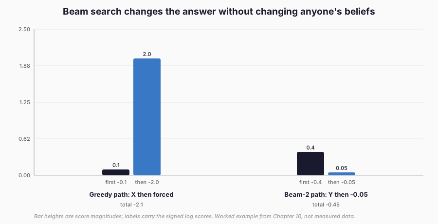
Figure 2. The two paths as score magnitudes with signed labels. Greedy commits at the first step and pays later; the beam survives the first step and wins overall. Worked example, not measured data. The implementation’s tests check ranking, width, tie-breaking by token id, completed-versus-truncated handling, and this exact greedy/beam divergence.
Length bias
Raw log probability accumulates one non-positive term per token, so longer sequences start at a disadvantage. A length penalty such as
Length also interacts with correctness. Longer sequences give error more chances to compound: in the E3 precursor, the baseline’s exact match by oracle output length falls from 0.95 at length 4 to 0.38 at length 8 (mean over seeds; the full bands are reported below). Truncation is the extreme case: a hypothesis cut off at the length limit is counted as wrong, and the truncation rate is reported separately (zero in this experiment, which is itself a finding about the length settings).
Exposure bias
Teacher forcing trains the student on reference prefixes. Inference feeds the student its own predictions. When an early prediction is wrong, every later prediction is conditioned on a context the student never trained on. Errors compound, and token accuracy overstates sequence correctness.
The E3 precursor measures both sides on validation data. Teacher-forced token accuracy is 90.0–97.6%; free-running exact match is 47–85% depending on seed, a gap of 12–43 percentage points. A sharper test forces the first output token to be wrong and measures completion: across all checked cases the completion rate is 0.0, while forcing the correct first token completes correctly 60–85% of the time (0.60–0.66 on the hard seed 2, 0.76–0.85 elsewhere). A single wrong first token destroys the sequence on this task. That is error propagation made visible, not a claim about all sequence tasks.
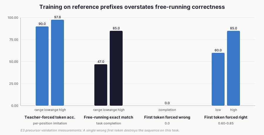
Figure 3. The exposure gap as ranges: per-position accuracy under teacher forcing against whole-sequence completion when free-running, plus the forced-first-token probe. E3 precursor validation measurements.
Scheduled sampling — mixing reference and model-generated prefixes during training — is a proposed mitigation. It changes the training distribution toward inference conditions at the cost of biased gradients and extra complexity. A related family, professor forcing and other adversarial prefix matchers, tries to make hidden states indistinguishable across the two regimes; they add a discriminator and its instability to the experiment. None of these removes the underlying mismatch for free: any prefix drawn from the student is itself a function of an unfinished model, so the “inference condition” being matched moves during training. This chapter does not implement any of them; Chapter 20 revisits on-policy learning where the idea belongs. The honest baseline is to report the gap — teacher-forced token accuracy beside free-running exact match — rather than to assume it away.
The E3 precursor task
The experiment uses a self-created symbol task, not language. Inputs are random strings over {A, B, C, D} (lengths 4–8); the oracle output reverses the string and applies the complement map (A↔D, B↔C). The mapping is deterministic and checkable, the vocabulary has 7 ids (PAD, BOS, EOS, four symbols), and all splits are disjoint by construction with rejection of cross-split duplicates.
The design deliberately avoids the usual confounds: no external corpus, no pretrained weights, no copyrighted text, no personal data. Lengths vary so that length bias is measurable; the space (87,296 pairs: 4^4+4^5+4^6+4^7+4^8) is large enough that disjoint splits keep the same length mix. A protocol amendment records why the minimum length moved from 2 to 8’s lower bound of 4: the length 2–3 space holds only 80 pairs, so guaranteeing disjointness starved later splits of short sequences. The amendment predates the controlled run and changes no result.
The teacher is a GRU encoder-decoder (embedding 16, hidden 64); the student uses embedding 8 and hidden 24. Both train with Adam, batch 64, up to 60 epochs, patience 10, ground-truth validation selection. The teacher is trained first, frozen, and then used for target generation (beam width 5, length penalty 0, max length 12, temperature 1). The test set is used once.
| Arm | Student supervision |
|---|---|
| A-hard | Cross-entropy on ground-truth targets |
| B-token-kl | Teacher-first KL at ground-truth prefixes, T=2, teacher-only |
| C-seq | Cross-entropy on teacher beam top-1 targets |
| D-seq-filtered | Cross-entropy on beam targets where the teacher output is oracle-correct, else ground truth (predeclared) |
Arm B is pure teacher signal, mirroring the E1 KL-only reference. Arm D’s filter uses training inputs only; the filtered fraction is reported.
What the precursor found
The teacher is strong: 99.1-99.6% token accuracy on the test inputs. Its beam outputs are oracle-correct on 99.8% of training inputs (filter rate 0.9975), which makes D very nearly a replication of C rather than a distinct comparison. That is reported, not hidden.
| Arm | Greedy exact (%) | Beam exact (%) | Agreement (%) | Token NLL |
|---|---|---|---|---|
| A-hard | 67.87 ± 16.80 | 69.63 ± 16.88 | 66.90 ± 16.04 | 0.18 ± 0.09 |
| B-token-kl | 46.53 ± 29.76 | 49.07 ± 29.37 | 45.87 ± 28.82 | 0.25 ± 0.14 |
| C-seq | 69.43 ± 14.25 | 71.97 ± 13.90 | 68.47 ± 13.58 | 0.17 ± 0.07 |
| D-seq-filtered | 65.43 ± 18.70 | 67.77 ± 17.03 | 64.50 ± 18.00 | 0.18 ± 0.09 |
Three patterns matter, and none of them is a universal ranking.
First, pure token-level KL without any hard labels is substantially worse than the baseline (−21.3 pp), with the largest seed spread of any arm. Matching the teacher’s distributions was not enough here. One plausible reading is that, without grounding in task labels, the student drifts; the experiment does not isolate the cause. This mirrors the E1 lesson that the objective defines what is optimised, and it is the strongest negative result in the chapter.
Second, sequence-level supervision roughly matches the baseline (+1.57 pp for C, within the seed spread). Training on the teacher’s single best sequence neither helps nor hurts much when the teacher is near-perfect and its outputs nearly equal the references — which is exactly when sequence distillation should be expected to add little.
Third, beam decoding helps every arm by 1.8-2.5 pp over greedy (A +1.76, B +2.54, C +2.54, D +2.34), at the cost of the beam search itself. The teacher’s beam outputs are the training targets and the agreement reference, so agreement tracks accuracy closely by construction.
Length bands show the compounding clearly for the baseline: exact match is 0.95 at length 4, 0.93 at length 5, 0.83 at length 6, 0.65 at length 7, and 0.38 at length 8. Longer sequences are harder for every arm, including the teacher-supervised ones.
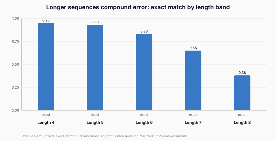
Figure 4. Baseline exact match falls from 0.95 at length 4 to 0.38 at length 8; every arm shows the same compounding pattern (per-arm levels differ). E3 precursor measurement, not a universal law.
Why each metric exists
Oracle exact match is the primary metric because the task has an oracle: the output either equals the correct transformation or it does not. Token accuracy and token NLL are diagnostic: they show whether the model learned local conditionals, but a model can score 99% of tokens right and still fail most sequences, as the length bands demonstrate. Sequence NLL preserves the likelihood scale for comparison with perplexity-style results; token NLL divides it out. Teacher agreement measures imitation of the beam output and is reported beside correctness precisely so the two cannot be confused. Length statistics, truncation rate, and empty-output rate exist to catch degenerate strategies — a student that always emits EOS would have excellent length statistics and zero correctness, and the table would show both facts at once.
Correctness versus imitation
Teacher agreement — exact match to the teacher’s beam output — is reported for every arm, but it is a diagnostic, not the headline. On this task the teacher is near-perfect, so agreement and correctness move together; that is a property of this teacher, not a reason to substitute one metric for the other. The primary metric is oracle exact match: does the student’s sequence equal the correct transformation, regardless of what the teacher produced.
The filtered arm illustrates the distinction. Because the filter almost never triggered, D trained on nearly the same data as C, and its score was within the seed spread of C’s (65.43% against 69.43% greedy exact match). Had the teacher been weaker, D would have mixed two different supervision sources, and its result would need to be read as a property of the mixture, not of “sequence distillation” in general.
Filtering is a comparison, not a cleanup
Arm D filters teacher targets by oracle correctness and falls back to ground truth where the teacher is wrong. The design needs care to stay honest. First, the filter may only use training inputs and training labels — never validation or test outcomes, and never the student’s own performance. Second, the filter rate is part of the result: at 100% the arm replicates C, at 0% it replicates A, and anything in between is a mixture whose performance cannot be attributed to a single supervision type. Third, filtering on correctness discards exactly the examples where the teacher is most informative about its own failure modes; a “quality” filter can remove the hardest and most useful training signal. In this experiment the filter rate was 99.8%, so D very nearly replicates C and is reported as such. A reader who sees near-identical C and D rows should conclude that the teacher was near-perfect here, not that filtering is free in general.
Cost and query economics
Every student has 5,127 parameters and a 20,508-byte artefact. Training took roughly 10–15 s per arm-seed on CPU; teacher beam generation for all 3,600 training inputs cost 24.1 s total and is reported separately from student training, because target generation is part of the method’s bill. Greedy latency is measured per example by repeated timed decodes with warm-up; beam-5 multiplies decoding work by roughly the beam width, plus the cost of maintaining and pruning hypotheses. These are local diagnostics, not provider prices: a hosted API would charge per token or per request under its own metering, and caching or batching policies would change the numbers. Peak process memory (484.7 MB cumulative) includes the Python and PyTorch runtime, not model tensors alone.
Rights and generated text
Teacher-generated sequences are model outputs. They can reproduce memorised training text, encode personal or confidential inputs, and carry contractual restrictions on storage, training use, redistribution, and competing-model development. The risk scales with the generator: a 7-token vocabulary on procedural symbol strings cannot memorise anything, but the same pipeline pointed at a large language model could emit training data verbatim.
The record-keeping does not change with scale. Every generated target in this experiment carries a provenance record: input hash, teacher and run identity, beam width, length penalty, max length, EOS/truncation status, output hash, and timestamp. What changes with scale is the legal review that record supports. A threshold question for any larger programme is whether the teacher’s terms permit training on its outputs at all; Chapters 36–39 develop that analysis, and no experiment in this book proceeds without a recorded answer. Synthetic does not mean unrestricted.
The experiment used only self-created data and models under RM-104, which
authorises train_and_evaluate_e3_precursor and nothing else. No rights record
was changed.
When sequence distillation helps or fails
Sequence-level supervision is most plausible when the teacher’s mode is informative: the beam output concentrates useful choices, avoids the harder regions of the target space (Kim and Rush report the mode holding 16.9% of the mass for their Seq-KD student versus 0.9% for the baseline), and greedy decoding becomes viable. It fails or adds nothing when the teacher merely reproduces the references (as here), when beam search truncates or degrades the targets, when length bias selects short but wrong outputs, or when exposure bias makes free-running behaviour diverge from teacher-forced metrics.
The E3 precursor lands in the middle: token-level KL alone hurts, sequence targets match the baseline, and the measurable differences are small against large seed variation. That is a valid negative-to-null result, and it sets up the questions Chapters 17–20 must answer at language-model scale.
A practical reading for the engineer: start with the hard-label baseline and a probability-matching arm, as Chapters 05–06 recommend. Add sequence-level targets when the teacher’s mode is informative and beam search is affordable — Kim and Rush’s tenfold decoding speedup is the prize, but it was measured on their models, not promised in general. Add token-level KL when the teacher’s per-position distributions are trustworthy; on this task they were not enough on their own. Keep every variant’s targets, filters, and decoding budgets in the provenance record, because a sequence experiment is won or lost in those details long before the final metric is read.
Limits of this chapter’s evidence
- Set-up: one self-created symbol-transformation task and small GRU models, with a near-perfect teacher whose beam outputs almost always equal the references.
- Measurements: three seeds, with standard deviations of 14–30 percentage points on exact match. The differences between A, C, and D are within that spread. Latency, training time, and memory are local diagnostics, not prices.
- Implementation: the filtered arm used beam targets for 99.8% of inputs, so it is not a distinct comparison. Teacher agreement tracks accuracy by construction here. Scheduled sampling and related mitigations were not implemented.
- Scope: the cause of the token-level KL arm’s deficit is not isolated. The Kim and Rush results come from their translation tasks and were not replicated. Nothing here establishes behaviour at language-model scale.
Preparing for multi-teacher distillation
Chapter 10 used one teacher. Chapter 11 asks what happens with several: how to aggregate their outputs, when the ensemble beats the best single teacher, how to measure disagreement, and when incompatible output spaces or licences forbid aggregation. The E3 precursor stays single-teacher by design; its provenance records and per-arm costs are the inputs that a multi-teacher comparison would need.
References
Kim, Y. and Rush, A. M. (2016). Sequence-Level Knowledge Distillation. Proceedings of the 2016 Conference on Empirical Methods in Natural Language Processing, pp. 1317–1327. https://aclanthology.org/D16-1139/