Self-Distillation
Can a model improve by learning from a version of itself? Born-again self-distillation with soft targets, pseudo-label self-training with confidence thresholds, confirmation bias measured as error inheritance, and a controlled E1 comparison including a hard-teacher control and an external-teacher reference.
Chapter 20 changed where training states come from. This chapter changes who the teacher is: an earlier generation of the student itself. The question is sharper than it looks:
Can a model improve by learning from a version of itself, and when is that just self-training or confirmation bias?
The chapter’s answer, measured on a four-class spiral with tiny MLPs, is that the words matter more than the weights. Soft supervision from a flawed same-arch teacher is associated with a small mean gain (+0.032 held-out accuracy, below the baseline on one of three seeds). Hard pseudo-labels from the same teacher, mixed with ground truth, give a similar mean gain (+0.022, also below the baseline on one seed) while visibly importing the teacher’s confident errors.
Hard supervision from that teacher alone, with no ground truth anywhere, collapses correctness from 0.65 to 0.39 while reporting the best calibration in the study. And an external teacher about seventy-six times larger teaches worse than plain labels on the mean, as the E1 comparisons in Chapter 06 found, though it edged ahead on one seed. None of these outcomes is a success story about self-improvement. All of them are legible — which is the point: when the teacher is yourself, every mechanism is auditable, and the audit is the chapter.
Can a model teach itself?
“Teaching itself” sounds like getting something for nothing, and in one strict sense it is: no new ground-truth label enters the pipeline at any point. What enters instead is structure — the teacher’s distribution over answers, its ranking of alternatives, its confidence — applied to inputs the student has or has not seen labelled. Whether that structure helps depends on what it is and where it is applied, and the literature’s two answers must not be confused: self-distillation transfers soft predictions from a frozen earlier generation; self-training assigns hard pseudo-labels to unlabelled inputs and trains on them. One smooths, the other decides. The chapter keeps them in separate arms, separate losses, and separate verdicts.
What counts as self-distillation?
A teacher derived from the same model family, architecture, or weights supervises the student — that is the whole definition, and it is deliberately narrower than “any training involving two networks”. Four variants appear in the literature and in this chapter’s comparison table: born-again networks (Furlanello et al., 2018, P-025), where generation G0 is frozen and a freshly initialised same-architecture G1 trains on G0’s soft outputs plus ground truth; snapshot distillation, where the teacher is an earlier checkpoint of the same run; same-family distillation across sizes; and self-distillation with augmentation, where the teacher labels transformed inputs. What unites them is frozen-teacher soft supervision with shared lineage. What distinguishes each case is stated per case: teacher version, student version, labels, loss — never assumed from the family name.
Six ways to supervise, compared
| Approach | Teacher identity | Label source | Data source | Soft vs hard | New unlabelled inputs? | Teacher frozen? | Student generates states? | Main failure mode |
|---|---|---|---|---|---|---|---|---|
| Supervised (Arm A) | none | ground truth L | L | hard | no | n/a | no | label noise ceiling |
| External KD (Arm E, Ch06) | big MLP, other arch | ground truth + big-teacher soft | L | both | no | yes | no | confident teacher adds nothing |
| Born-again (Arm B) | frozen G0, same arch | ground truth + G0 soft | L | both | no | yes | no | inherits teacher bias softly |
| Pseudo-label self-training (Arm C) | frozen G0, same arch | ground truth + G0 hard on U | L + U | hard | yes | yes | no | confident errors amplified |
| Hard-teacher control (Arm D) | frozen G0, same arch | G0 hard on L only | L | hard | no | yes | no | echo chamber, no grounding |
| On-policy (Ch20) | frozen external teacher | teacher conditionals on student prefixes | evolving student states | soft | n/a (states, not labels) | yes | yes | staleness, sampling cost |
Read down the “New unlabelled inputs?” column: only self-training adds inputs the labels never described. Read across the “Soft vs hard” row: only born-again and external KD soften. The table is the chapter’s terminological contract — every later claim cites a row.
KD-026 — Self-distillation
Self-distillation (KD-026): a teacher derived from the same model family, architecture, or weights supervises the student; distinct from an external-teacher setup. In this chapter’s experiment the teacher G0 and the student G1 share the exact architecture (2→32→4 MLP, 228 parameters) and differ only in initialisation seed-stream position and supervision: G0 saw hard labels alone; G1 sees hard labels plus G0’s softened distribution. Furlanello et al. report that such born-again students can surpass their teachers on CIFAR (P-025); our E1 study finds a small mean gain (+0.032) with a sign flip on one of three seeds — suggestive, not established, and reported with the seed-level values visible.
KD-027 — Self-training
Self-training (KD-027): a model labels unlabelled data and trains on those pseudo-labels; it may or may not use a distillation objective. Our Arm C uses no distillation objective at all — hard cross-entropy on hard pseudo-labels — which is precisely why it belongs to KD-027 and not KD-026. Pseudo-labels may be correct, incorrect, overconfident, class-biased, duplicative, or informative about previously unseen regions; the audit in Section 27 measures each property separately instead of averaging them into a single “pseudo-label quality” that would hide the structure. Xie et al. (P-026) show this family at ImageNet scale with noise and augmentation; our demonstration is deliberately small, deterministic, and fully auditable.
The information-source problem
H3 first, because it governs every table that follows. Training G1 on G0’s outputs cannot create ground-truth information: the labels in L are the only facts about the spiral in the building, and G0’s 228 parameters already summarised them once. Candidate mechanisms for any observed gain are therefore restricted to: soft-target regularisation (smoother, instance-specific targets), altered optimisation (different gradient path, same minimums), exposure to new inputs (the unlabelled pool U, whose inputs are new even though their labels are not), and selection effects (thresholding keeps easy examples).
The experiment is designed to separate the first two (Arm B vs Arm A: same inputs, added soft targets), the third (Arm C vs Arm A: added inputs, hard targets), and the cost of the fourth (Arm D: teacher hard targets alone). If none separates cleanly, the chapter reports that — and on correctness, B and C barely separate from each other (+0.679 vs +0.669 with overlapping spreads).
Born-again neural networks
The born-again recipe (P-025) is minimal: train G0 to convergence on hard labels; freeze it; initialise G1 from scratch with the same architecture; train G1 on hard labels plus G0’s softened outputs; optionally iterate to G2. Furlanello et al. report DenseNet born-again generations beating their teachers on CIFAR-10/100, and explore two refinements — confidence-weighted teacher max and dark knowledge with permuted predictions — to isolate which part of the teacher signal helps.
Our study implements the plain form only: identical architecture, frozen G0, mixed hard/soft objective, no teacher-side tricks. That restraint is deliberate. The chapter’s question is whether the mechanism transfers to a setting where every confound is measured, not whether the paper’s headline number replicates — it cannot, at this scale, and the chapter never claims otherwise.
    flowchart LR
  G0[train G0 on hard labels] --> F[freeze G0]
  F --> G1[train fresh G1: hard labels + G0 soft targets]
  G1 -->|optional| G2[repeat as G1's student]
Figure 1. The born-again loop: the supervision changes, nothing else does — which is the whole logical force of the design.
A teacher and a student with the same architecture
Example A. G0 is a 2→32→4 MLP (228 parameters) trained 3000 updates on 1,200 labelled spiral points, best-validation restored (val 0.86/0.90/0.77 across seeds; test 0.634/0.624/0.683). G1 is a freshly initialised 2→32→4 MLP — same layer widths, same count, different random start, verified unequal to G0’s weights. The supervision differs, not the capacity: G1 sees the same 1,200 labels plus G0’s temperature-2 softened distribution over them.
There is no compression here, no bigger mind pouring into a smaller one. If G1 beats G0, the gain must come from the form of the supervision — soft instead of hard — because nothing else changed. That is the entire logical force of the born-again design, and the reason the external-teacher arm exists as its foil.
Deriving the born-again distillation objective
For a labelled example (x, y) with frozen teacher G0 and student G1:
\(L = (1-\lambda) L_{CE}(y, p_{G1}) + \lambda T^2 D_{KL}(p_{G0}^{(T)} \mid\mid p_{G1}^{(T)})\)
with \(T = 2\), \(\lambda = 0.5\) — the book’s canonical mixed objective from Chapter 05, unchanged. The hard term anchors G1 to ground truth; the soft term pulls G1’s tempered distribution toward G0’s, scaled by \(T^2\) so the gradient magnitude survives temperature smoothing (Chapter 05’s derivation, not repeated). The teacher is detached: no gradient flows into G0, ever — the implementation freezes it and the tests assert frozen weights and absent teacher gradients. Limiting cases: \(\lambda = 0\) recovers Arm A exactly; \(\lambda = 1\) is KL-only supervision; \(T = 1\) sharpens the teacher toward its own argmax. The chapter runs the predeclared middle, not a sweep.
Hard targets versus soft teacher distributions
Arm D exists to isolate target type on matched inputs: same 1,200 labelled examples as Arms A and B, but the targets are G0’s hard predictions — no ground truth anywhere, no softness anywhere. If soft targets carry the benefit, D should underperform B; if merely training longer or seeing teacher-flavoured targets sufficed, D should track B. What happens instead is more instructive than either prediction: D collapses to 0.385 mean accuracy (0.304/0.310/0.542 per seed), far below its own teacher’s 0.647.
Hard imitation of a flawed teacher without ground-truth anchoring does not preserve the teacher — it amplifies the flaws. B’s soft targets on the same inputs, anchored by the same hard labels B also sees, reach 0.679. The comparison is clean because the inputs are identical; the conclusion is narrow for the same reason. Do not read it as “soft always beats hard” — read it as “hard imitation without grounding fails here, measurably”.
Instance-specific label smoothing
Example B. Uniform label smoothing replaces a one-hot target with \((1-\epsilon) y + \epsilon u\) for uniform \(u\): every example gets the same smoothing, regardless of content. Born-again soft targets replace it with \((1-\lambda) y + \lambda p_{G0}(\cdot|x)\): the smoothing distribution depends on the example — confident where G0 is confident, diffuse where G0 is uncertain. Zhang and Sabuncu (P-069) formalise this as amortised MAP inference with instance-specific regularisation, and argue that predictive dispersion across examples matters alongside per-example uncertainty.
Our test of the interpretation is behavioural, not formal: if G0’s softness merely relabelled easy examples, Arm B would match Arm A everywhere including calibration. Instead B gains +0.032 accuracy while losing calibration (ECE 0.161 vs 0.126) — soft targets reshaped which examples the student gets right, not just how confidently it gets them. The smoothing interpretation survives; the “smoothing always calibrates” corollary does not, at least here.
Building a pseudo-labelled dataset
Example C. The unlabelled pool U holds 2,000 fresh spiral draws per seed; their oracle labels exist but are locked in the audit vault — the pseudo-labelling function does not even accept a labels argument, so leakage is structural, not procedural. Frozen G0 scores every U input; max-probability is the confidence; the predeclared rule keeps predictions at or above \(\tau = 0.8\) (minimum 100 kept, else Arm C is declared INCOMPLETE — no silent lowering). Measured yields: 210/200/206 kept (10–10.5%), class counts heavily skewed (seed 11: 99/7/75/29).
The threshold was set from a seed-11 pilot (τ = 0.9 kept under 2%), disclosed in the protocol — calibration before freezing, not tuning after results. Walk through one: a seed-11 U point G0 calls class 0 at 0.93 confidence. Kept (0.93 ≥ 0.8), trains as a hard class-0 target, joins 1,200 ground-truth rows in Arm C’s batches. The audit says class-0 pseudo-labels were 100% correct on this seed (99/99) — this one almost surely was too. Contrast a seed-11 point G0 calls class 2 at 0.97: also kept, but its band ([0.95,0.99)) was only 42.9% correct. Same rule, same threshold, opposite lesson about what confidence means.
Confidence thresholds and selection
The threshold trades quantity against supposed quality, and the audit shows the supposition failing in an instructive direction. Seed-11 correctness by confidence band: [0.8, 0.9) holds 178 of 210 selected at 96.0% correct; [0.9, 0.95) holds 18 at 83.3%; [0.95, 0.99) holds 14 at 42.9%; nothing clears 0.99. Higher confidence predicts lower accuracy in this pool — G0 is most confidently wrong exactly where a threshold trusts it most. Class balance is worse: class 1 contributes 7 of 210 selected on seed 11. The chapter states the consequence plainly: thresholding selected easy, already-learnable regions and amplified the teacher’s confident mistakes, which is why Arm C matches but does not beat Arm B despite 200 extra training inputs.
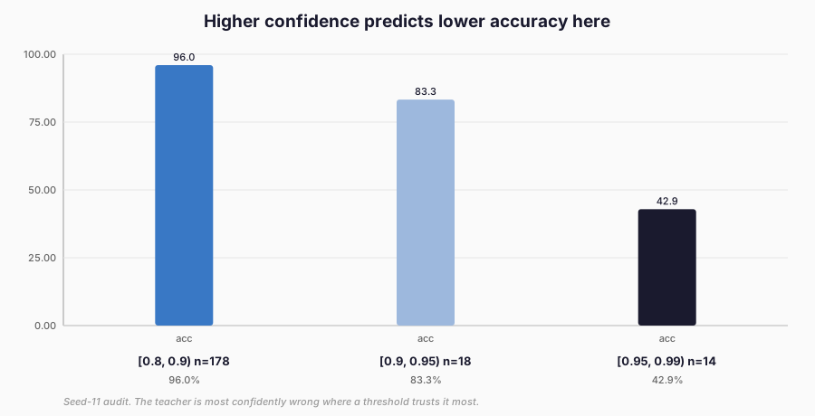
Figure 2. Seed-11 pseudo-label accuracy by teacher confidence band, with counts. The threshold trusts exactly the band where the teacher is most wrong. Chapter 21 audit measurements.
The confirmation-bias problem
Confirmation bias, operationalised: the student inherits the teacher’s errors, then the evaluation counts them as the student’s own findings. Measurement, not metaphor: on seed 11, Arm B introduces 31 new errors relative to G0 while sharing 284 and correcting 82 — the soft-target student mostly repeats G0 with modest repair. Arm D introduces 415 new errors, shares 281, corrects 85: hard imitation without grounding manufactures error at thirteen times Arm B’s rate while correcting no more.
Arm C sits between (pseudo-label accuracy 0.914/0.855/0.956 across seeds bounds how much error enters, and its ground-truth L component anchors the rest). Agreement statistics alone would call D (0.355–0.770 agreement with G0) “less distilling” than B (0.806–0.896); the error ledger says what agreement cannot — whose errors, and how many are new.
A high-confidence wrong-label example
Example D. Teacher logits [0,0,0,9.0] on an input whose oracle class is 1: max-probability ≈ 1.0, pseudo-label 3, wrong with total confidence. Under thresholding this example is always kept; under hard training its gradient pulls the student fully toward class 3; under soft training with \(T = 2\) the same logits spread meaningful mass onto the true class and the pull weakens. The fixture is hand-constructed and labelled as such — it demonstrates the channel (high confidence × wrong label → amplified error), while the seed-11 audit supplies the field evidence (14 such cases at ≥0.95 confidence, 42.9% band accuracy). One shows the mechanism can exist; the other shows it did.
The frozen E1 experiment
Run E1S-20261116T084945Z-222968, protocol 1.0 + recording-only
amendment A1, rights RM-113
(train_born_again_and_pseudo_label_e1, verified-permitted, gate
first). Fresh spiral draws, seeds 11/12/13: L train 1200, val 400,
test 1000; U pool 2000 with labels withheld (exact-overlap checks
pass; zero duplicates). G0 (student arch, hard labels, 3000 updates)
and a big external teacher (2→128→128→4, same recipe) frozen with
checkpoint hashes. Students: five fresh seed-matched inits per seed
(asserted equal), EXACTLY 3000 updates each, batch 64, Adam 0.01,
best-validation restore on each arm’s own objective after the full
budget — actual updates matched structurally, not by patience luck.
Held-out test evaluation only; test ledger appended; nothing tuned
on test outcomes. First full run superseded by A1 (missing
teacher-test-accuracy fields) and retained, not cited.
Supervised baseline
Arm A — hard labels on L, 3000 updates — is the reference every claim must beat, and it reproduces G0 exactly (0.634/0.624/0.683; identical by deterministic construction: same procedure, seed, init, data, and budget). This identity is a feature, not a bug: the baseline is generation zero, so every other arm measures a departure from it. A reaches 0.647 ± 0.032 with ECE 0.126 and Brier 0.475. Keep these three numbers in view; the rest of the section spends them.
Born-again training results
Arm B — hard labels plus frozen G0 soft targets — reaches 0.679 ± 0.008 (+0.032 over A; per-seed +0.051/+0.058/−0.013). The mean gap exceeds the seed spread on two of three seeds but flips sign on the third: suggestive, not established. NLL improves (0.838 vs 0.863) while ECE degrades (0.161 vs 0.126) — accuracy and calibration move opposite directions, repeating Chapter 06’s lesson that the KL arms trade one for the other. Brier improves slightly (0.460 vs 0.475). Teacher agreement with G0 is 0.806–0.896: B follows G0 closely, which is expected (it trains on G0’s distribution) and is reported as diagnostic, not achievement.
Self-training results
Arm C — hard labels plus thresholded G0 pseudo-labels — reaches 0.669 ± 0.027 (+0.022 over A; per-seed deltas +0.027/+0.075/−0.035). NLL 0.839, ECE 0.124 (essentially A’s calibration preserved), Brier 0.460. Pseudo-labels are 86–96% correct, so the error channel is narrow — and the gain is correspondingly narrow. The instructive contrast is with D, not A: the same teacher’s hard outputs, with ground-truth anchoring and selection, add a whisper; without anchoring, they destroy. Self-training here is safe but small, because the filter kept it safe (10% yield) and small (200 extra examples on 1,200).
Held-out correctness
Example F, the actual comparison (frozen run E1S-20261116T084945Z-222968):
| Seed | A supervised | B born-again | C self-train | D hard-teacher | E external |
|---|---|---|---|---|---|
| 11 | 0.634 | 0.685 | 0.661 | 0.304 | 0.580 |
| 12 | 0.624 | 0.682 | 0.699 | 0.310 | 0.629 |
| 13 | 0.683 | 0.670 | 0.648 | 0.542 | 0.670 |
| mean ± SD | 0.647 ± 0.032 | 0.679 ± 0.008 | 0.669 ± 0.027 | 0.385 ± 0.136 | 0.626 ± 0.045 |
No arm was selected on test outcomes; the best seed is not the headline (means and spreads are). The directional hypotheses: H1 supported weakly (B > A on two seeds, mean +0.032, tight spread ±0.008); H2 supported weakly (C > A on two seeds, +0.022); H3 holds structurally — D’s collapse with identical inputs to B shows the supervision form, not the inputs, drives the failure. The external teacher (E, 0.626) loses to plain labels on the mean (it edges ahead on seed 12), consistent with E1’s classical result: bigger is not better here, and its inclusion as a reference arm is what lets the chapter say so with numbers instead of scepticism.
Calibration and Brier score
Example E. ECE with 15 equal-width bins: A 0.126, B 0.161, C 0.124, D 0.065, E 0.100. Brier (mean squared error vs one-hot): A 0.475, B 0.460, C 0.460, D 0.691, E 0.471. Two readings matter. First, D reports the study’s best ECE (0.065) alongside its worst accuracy (0.385) and worst Brier (0.691) — calibration without correctness is the degenerate case the chapter warned about in Chapter 05, now measured: D’s collapsed predictions are confidently concentrated on two classes (seed-11 per-class accuracy 0.684/0.000/0.212/0.320), and ECE rewards the concentration. Second, B’s accuracy gain costs calibration while C preserves it — soft targets sharpen, hard pseudo-labels on top of ground truth do not. NLL agrees (B 0.838, C 0.839 vs A 0.863). Report all three; trust none alone.
Prediction diversity
Prediction histograms per arm are full-support except D’s collapse (unique predicted classes: 4/4/4/3–4/4). Entropy of the predicted distribution is highest for the collapsed arm on two seeds — garbage is diverse, repeating Chapter 20’s warning verbatim, so the chapter states it verbatim: diversity without correctness is noise. The multi-generation fixture (below) adds the directional prediction: repeated self-distillation concentrates mass on the teacher’s mode, reducing diversity generation over generation while accuracy moves ambiguously. Measured: B’s agreement with G0 (0.806–0.896) exceeds its agreement gain over A — imitation dominates, acquisition is the residue.
Error inheritance and correction
The error ledger is the chapter’s core table (seed 11; other seeds in evidence). B: 31 new, 284 shared, 82 corrected. The corrections exceed the introductions more than twofold — soft supervision repairs more than it breaks, which is the entire case for born-again in one row. D: 415 new, 281 shared, 85 corrected — hard imitation breaks nearly five times what it repairs, and thirteen times what B breaks.
C’s pseudo-label audit bounds its channel: 86–96% correct inputs, high-confidence errors counted explicitly (seed-11 illustration in § worked example). Note what agreement would have said: D agrees with G0 least (0.355), B most (0.843) — agreement ranks the arms by imitation fidelity, and imitation fidelity here is inversely related to correctness.
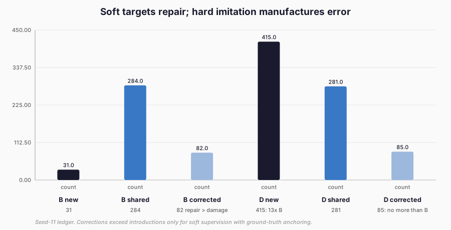
Figure 3. Seed-11 error counts against teacher G0: shared errors dominate both arms, but only the born-again arm corrects more than it invents. Frozen E1 measurements. That inversion is why the book measures correctness independently (KD-032), in every chapter, without exception.
Multi-generation stability
A deterministic fixture, labelled as such — not a third training campaign. Take a 4-class teacher distribution [0.70, 0.20, 0.07, 0.03] and distil with \(\lambda = 0.5\), \(T = 2\) for two generations, each student becoming the next teacher. Generation 1’s target mixes the one-hot label with the teacher; generation 2’s target mixes the one-hot label with generation 1’s sharpened output. Arithmetic (verified in tests): each generation concentrates mass on the teacher’s top class and thins the tail — instance smoothing with a shrinking kernel.
If the top class is correct, later generations look increasingly confident and correct; if it is wrong, later generations look increasingly confident and wrong. That is the whole stability question in four numbers: self-distillation is a confidence ratchet, and ratchets do not know what they are tightening. Whether real G2 training follows the fixture is not measured here — stated, not hidden.
Runtime and lifecycle cost
Student arms cost 1.3–2.0 s each; G0 1.4 s, big teacher 3.8 s per seed; whole study 40.5 s wall. Teacher soft-target caching is counted in batched forwards; pseudo-labelling is one G0 forward per U input. Full lifecycle vs marginal: G0’s training is paid once and amortised over every student it teaches (here: four students per seed); the marginal student cost is ~2 s. The chapter declines the “self-distillation is cheap” moral anyway: cheap is measured against budgets that matter, and at this scale every arm is cheap — the cost table exists to show the accounting, not to declare a winner. No provider pricing exists; none is invented.
Self-distillation versus external teachers
Arm E — big-teacher soft targets (2→128→128→4, test accuracy 1.000/1.000/0.999) plus hard labels — reaches 0.626 ± 0.045, below the supervised baseline and below both self-distillation arms. The teacher is nearly perfect and nearly useless: its confident, near-one-hot distributions carry little beyond the labels, while G0’s softer, flawed distributions carry usable dark knowledge — exactly the capacity-mismatch argument from Chapters 03 and 06, now with the sign flipped in self-distillation’s favour.
The chapter’s answer to “when is an external teacher necessary” is therefore conditional, not tribal: necessary when the teacher knows things the labels do not contain (not here — the spiral labels are complete); unnecessary, even harmful, when the teacher merely restates them more confidently. Use the small flawed teacher you can audit over the large perfect one you cannot — on this task, with these numbers.
Rights, provenance, and limits
Every generation carries identity, parent, architecture, parameter
count, init seed, data fingerprint, config hash, checkpoint hash,
budget, and rights record (RM-113
train_born_again_and_pseudo_label_e1, verified-permitted, gate
first); students are freshly initialised per arm (asserted equal
within seed); pseudo-labels carry teacher version and threshold;
oracle U labels never enter training (the selection function has no
labels parameter — verified by signature test).
Limitations, without softening: one synthetic 2-D task, three seeds, tiny MLPs; τ and budget set from a seed-11 pilot (disclosed); G0 quality measured not tuned; A replicates G0 by construction; cross-seed prediction agreement not measured; no replication, no independent review. The strongest caveat first: with three seeds and sign flips on seed 13 (B) and seed 13 (C direction), neither improvement is established. What is established is that the supervision, not the inputs, drives D’s collapse; D differs from B in both softness and anchoring, so separating soft-vs-hard from anchored-vs-pure would need an arm that varies one of them alone.
Preparing for preference distillation
Selection (Chapter 19) filters whose outputs to learn from; on-policy training (Chapter 20) changes where training states come from; self-distillation (this chapter) changes who teaches. What none of them changes is what counts as better: all three optimise imitation of a reference — labels, traces, or a previous self. The remaining lever is preference itself: learning, from comparisons rather than demonstrations, which of two behaviours is preferred.
Chapter 22 builds that signal — pairwise preferences, a Bradley–Terry model, and the DPO objective — and asks whether preferring is a different kind of teaching or just distillation with extra steps. The ledger this chapter leaves behind — soft versus hard, anchored versus pure, inherited versus corrected errors — is the vocabulary that question will be asked in.
References
Furlanello, T., Lipton, Z. C., Tschannen, M., Itti, L. and Anandkumar, A. (2018). Born-Again Neural Networks. ICML 2018. https://arxiv.org/abs/1805.04770
Zhang, Z. and Sabuncu, M. R. (2020). Self-Distillation as Instance-Specific Label Smoothing. NeurIPS 2020. https://arxiv.org/abs/2006.05065
Xie, Q., Luong, M.-T., Hovy, E. and Le, Q. V. (2020). Self-Training with Noisy Student Improves ImageNet Classification. CVPR 2020. https://arxiv.org/abs/1911.04252