Dataset Distillation
Dataset distillation optimises the training examples themselves so a small synthetic set can train a fresh student. This chapter derives the bilevel objective and gradient matching, compares trajectory and distribution matching, and runs a bounded E2-shape condensation demo.
Sixteen randomly chosen examples trained students to a mean held-out accuracy of 0.756 in this chapter’s experiment, against 0.807 for the full 1,200. Sixteen examples synthesised by dataset distillation reached 0.762, a difference from the random sixteen that sits inside the seed noise; on two of the three seeds the random subset did better. The method is real and the mathematics is sound, but on this task it had almost nothing to improve on, and the chapter reports that rather than a win.
Chapter 15 subtracted examples and reordered them. This chapter takes the stronger step: synthesise the training set itself. The question is:
Can a small synthetic dataset preserve enough information to train a student almost as well as the original data?
The central argument is that dataset distillation optimises the training examples so that a model trained on a small synthetic set behaves like one trained on a larger dataset. The output is a dataset, not a student — and that single distinction organises everything that follows. The chapter ends with a bounded demonstration whose honest result is weak: on a simple task, the condensed set’s mean accuracy is within seed noise of a random subset’s, and the condensation objective barely moves. A weak result with a controlled design teaches more than a strong result without one.
Distilling a dataset instead of a model
Model distillation, the subject of Parts I and II, transfers a teacher’s supervision into a smaller student’s weights. The dataset is fixed; the student moves. Dataset distillation reverses the roles: the student-training algorithm is fixed, and the dataset moves. A small set of synthetic examples — pixels that need not look like anything, labels that may be fixed or optimised — is adjusted until fresh students trained on it behave like students trained on the full source. The test of success is downstream: held-out correctness of students that never saw the source data, not the value of the optimisation objective that produced the synthetic set.
Three neighbouring ideas must not be confused with it. Synthetic data generation (Chapter 14) produces examples without optimising them against a training objective. Coreset selection chooses a subset of real examples; it never synthesises a pixel. Filtering (Chapter 15) removes rows. Dataset distillation alone creates training inputs by optimising them — and pays for that privilege in second-order compute, as this chapter measures.
KD-019 and the central idea
Dataset distillation (KD-019) is the synthesis of a compact dataset that trains a fresh model to approximate the performance or learning behaviour obtainable from a larger source dataset. The registry definition fixes four points. First, the optimised object is the dataset: examples and possibly labels — our demo fixes labels and optimises pixels only, a declared restriction (optimised soft labels can carry extra supervision, but they also entangle the distillation with the teacher’s output space, a complication the demo does not need).
Second, the consumer is a fixed training algorithm — gradient descent from stated initialisations for a stated budget. Third, the synthetic examples may differ arbitrarily from real data; nothing requires them to be plausible inputs. Fourth, the verdict is downstream held-out correctness of freshly trained students. A method that minimises its own matching loss while its students fail is a failed distillation with a well-optimised auxiliary metric — the volume-equals-value confusion of Chapter 14 in a new costume.
The bilevel optimisation problem
Let \(D_{\mathrm{real}} = \{(x_i, y_i)\}{i=1}^{N}\) be the source training set and \(D{\mathrm{syn}} = \{(\tilde{x}j, \tilde{y}j)\}{j=1}^{M}\) the synthetic set, with \(M \ll N\). Let \(A(D, \theta_0)\) be the model-training algorithm applied to dataset \(D\) from initial parameters \(\theta_0\). The inner loop trains on synthetic data, \(\theta^*(D{\mathrm{syn}}, \theta_0)\); the outer loop chooses the synthetic data to minimise training loss on real data:
\[ \min_{D_{\mathrm{syn}}} \; \mathbb{E}{\theta_0 \sim P{\mathrm{init}}} \left[ \; L_{\mathrm{real,train}} \left( \theta^*(D_{\mathrm{syn}}, \theta_0) \right) \; \right]. \]
Three things make this hard. Differentiating through many training steps is expensive and memory-hungry: the outer gradient flows through every inner update, so truncating the unrolling (as gradient matching does to a single step) trades fidelity for feasibility, and the chapter prices that trade explicitly. The expectation over initialisations matters: a synthetic set that teaches one initialisation may fail the next — Wang et al. (2018) evaluate multiple initialisation settings for exactly this reason, and our demo condenses against sixty different inits.
And the outer objective uses training loss on real data: the held-out test set must never enter synthetic-data optimisation, or the downstream evaluation is circular — a set tuned against its own exam proves nothing about teaching. Our runner enforces this by construction — condensation receives the training partition only — and a test asserts the manifest contains no test reference in the condensation configuration.
The exact bilevel problem is not solved here. Everything practical is an approximation: one-step surrogates, truncated unrolling, matching objectives that stand in for the outer loss. The chapter is explicit about which approximation it implements and what it gives up.
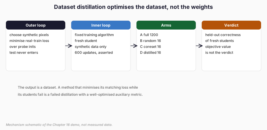
Figure 1. The two loops and the four arms. The inner loop is fixed; the outer loop moves pixels; fresh held-out students deliver the verdict. Mechanism schematic, not measured data.
Coresets and ordinary subset selection
The honest baselines come first. A random class-balanced subset takes \(K\) examples per class with a seeded shuffle — no intelligence, full reproducibility. A coreset applies a predeclared rule: ours keeps, per class, the \(K\) examples with the smallest total L2 distance to their classmates in pixel space (exact medoids over the 300 training members per class, ties by lowest index — deterministic, no seed, no test or validation contact). Both contain only real examples; neither synthesises anything.
The trade-off is instructive. Random subsets are unbiased but high-variance: seed 1’s random 16 reached 0.853 while seed 0’s reached 0.592. Coresets are stable (0.644–0.715 across seeds, the tightest spread of any arm) but mediocre (mean 0.670, worst of the four on aggregate — though not on every seed: it beats random on seed 0): medoids are the most typical examples, and typical examples are not the most teachable ones.
Typicality is a property of the source distribution; teachability is a property of the learning algorithm. A coreset optimises the first and hopes for the second. This chapter keeps both baselines because any synthesis method must beat selection before it can claim to be more than selection — and in our demo, the synthesis does not clearly do so.
Gradient matching
If a synthetic batch induces the same parameter gradients as a real batch, one gradient step on either batch moves the student the same way. That is the whole idea (Zhao et al., 2021): match gradients instead of unrolling training. Let \(g_{\mathrm{real}}(\theta) = \nabla_\theta L(D_{\mathrm{real}}; \theta)\) and \(g_{\mathrm{syn}}(\theta)\) likewise. The matching objective is:
\[ \mathbb{E}{\theta \sim P\theta} \left[ \; d\left(g_{\mathrm{syn}}(\theta), g_{\mathrm{real}}(\theta)\right) \; \right], \]
with \(P_\theta\) the distribution over probe initialisations. Our demonstration uses the simplest declared distance, \(d(g_s, g_r) = \|g_s - g_r\|_2^2\), flat over all parameters and summed over classes — not the paper’s per-layer normalised distances, and the chapter says so.
Implementation has three load-bearing details, each tested. First, real
gradients are detached fixed targets; the outer backward pass must not
differentiate through them. Second, synthetic gradients need
create_graph=True so the outer loss differentiates through the
gradient computation into the pixels — and the test suite verifies the
synthetic images receive nonzero gradients while the probe model’s
weights are byte-identical before and after (a model_mutated
assertion runs on every outer step). Third, labels are fixed: only
pixels move. The original paper explores more; the demo declares less
and checks what it declares.
A single outer step on seed 0 makes the mechanism concrete. Fresh probe (init seed 1000), real batches of 32 per class, synthetic 4 per class: per-class distances 0.00175/0.00182/0.00200/0.00191, total 0.00749, outer gradient norm on the pixels 0.00511. One SGD step (lr 0.1) nudges 16 images down that gradient and clamps to [0,1]. Nothing about the step is mysterious; the mystery the chapter refuses to manufacture is whether sixty such steps add up to a better dataset.
In this demo, they do not: the distance ends at 0.00502 on seed 0 and drifts slightly up on seeds 1 and 2. The objective is flat because the synthetic set starts from real images whose probe gradients already match. Gradient matching from a real-image initialisation on a tiny network has almost nothing to fix.
Why synthetic images receive gradients
Differentiating through a gradient computation surprises readers who
think of gradients as the end of the line. The chain is mechanical:
synthetic pixels → forward pass → cross-entropy → parameter gradients
(a differentiable function of the pixels via the forward pass) →
squared distance to fixed real gradients → scalar. Every arrow is
differentiable, so backward() on the scalar reaches the pixels. The
cost is second-order computation: the outer backward differentiates
through the inner gradient, roughly doubling the backward cost and
holding the inner graph in memory.
On our tiny CNN (372 parameters, 16 synthetic images) that is milliseconds; on a ResNet with thousands of synthetic images it is the reason dataset distillation is compute-limited — the limitation the evidence posture of this chapter promises to be frank about. Finite-difference checks in the test suite confirm the outer gradients point downhill on the distance; the failure of the distance to fall further is a property of the optimisation landscape, not of the implementation.
Training-trajectory matching
Gradient matching compares single steps. Trajectory matching (Cazenavette et al., 2022) compares destinations: train a probe on synthetic data for several iterations and minimise the distance between its parameters and the parameters of an expert trained on real data. Experts are pre-computed and stored — the paper’s key efficiency move — and the distilled set is optimised to steer fresh probes toward expert states across many steps rather than to imitate one gradient.
The trade-offs are direct. Trajectory matching sees longer-horizon behaviour and, in the paper’s experiments, handles higher-resolution data better; it costs expert-trajectory storage, multi-step unrolling, and tight coupling to the architecture the experts used. It is not implemented in this chapter. The contract requires a conceptual comparison, not a second optimisation system, and building one would break the compute ceiling that keeps this demo honest. The reader gets the derivation, the cost model, and the pointer — not a half-built trajectory matcher presented as a result.
Distribution matching
A third family skips gradients entirely and matches statistics: class-conditional feature means, for instance, minimising \(\sum_c \|\mu_c^{\mathrm{real}} - \mu_c^{\mathrm{syn}}\|_2^2\) over some feature map \(\phi\), where \(\mu_c\) is the mean feature of class \(c\) in each set. On the E2 shapes a pixel-space version is easy to picture: the mean horizontal-stroke image is a grey horizontal band ( strokes at all positions averaged), and a synthetic set whose class-means reproduce those bands matches the first moment exactly. It is cheap, stable, and conceptually clean — and it proves nothing about downstream students. Equal means do not imply equal trainability: a synthetic set can match every class mean while containing no single image the student algorithm can learn stroke position from, because the mean of strokes at all positions is a blur at no position.
A student trained on blurs learns blurs. The chapter treats distribution matching as a mechanism with stated assumptions, not as an implemented arm: the moment it matches is a property of the source, and teachability is a property of the learning algorithm — the same distinction the coreset result demonstrates empirically. One matching objective per demo is enough; three would be a catalogue, and catalogues are not evidence.
Designing the tiny condensation experiment
Source: the E2 four-class shape task (12×12 single-channel images, horizontal/vertical/diagonal strokes plus Gaussian noise), regenerated under a frozen D1 protocol — 1,200 train, 400 validation, 1,000 test per dataset seed (0, 1, 2) — without touching historical E2 records. Compression: 16 synthetic examples (4 per class), ratio \(R = 75\) by count, 700,800 → 9,344 bytes by storage. Arms: A full-data, B random balanced 16, C medoid coreset 16, D gradient-matched 16. Condensation: 60 outer steps, real batches of 32 per class, SGD lr 0.1 on pixels, fresh probe init per step from a pool disjoint from evaluation inits.
The student everywhere — probe and fresh — is the E2 small CNN (channels (4,8), ~372 parameters), trained with Adam 0.002, batch 32, and best-validation checkpointing that always runs the full 600-update budget before restoring, so the checkpoint rule cannot unmatch the budgets it selects among. Evaluation inits equal the dataset seed (identical across arms within a seed); condensation inits live above 1000 plus a per-seed offset. The two pools never intersect, and the config records the policy in one line so the separation is checkable, not claimed.
The Chapter 15 lesson is structural, not decorative: every arm trains
for exactly 600 optimiser updates (batch 32, Adam 0.002, seeded
replacement sampling), with best-validation checkpointing that runs the
full budget before restoring. A test reads the manifest and asserts all
twelve runs report 600. Updates matched; unique exposures measured
(and differing by construction: the full arm sees ~1,200 uniques, small
arms revisit 16). Rights: RM-108
(optimise_and_evaluate_distilled_dataset, verified-permitted), gate
passed before any optimisation. No external data, models, or inference.
Comparing full, random, coreset and distilled sets
The frozen run (D1-20261115T161713Z-8bbf14) trained 12 students (4
arms × 3 seeds). Held-out accuracy (primary), per dataset seed:
| Seed | A-full (1200) | B-random (16) | C-coreset (16) | D-distilled (16) |
|---|---|---|---|---|
| 0 | 0.698 | 0.592 | 0.644 | 0.671 |
| 1 | 0.782 | 0.853 | 0.651 | 0.832 |
| 2 | 0.942 | 0.824 | 0.715 | 0.782 |
Aggregates: A 0.807 ± 0.124, B 0.756 ± 0.143, C 0.670 ± 0.039, D 0.762 ± 0.082. Cross-entropy follows (A 0.516, B 0.664, C 0.766, D 0.654); ECE is lowest for the coreset students (0.061 against 0.105–0.139 elsewhere), a calibration footnote, not a success — the coreset is confidently mediocre where the other small arms are uncertain and occasionally right. Every arm ran exactly 600 updates (asserted per run in the manifest, not merely configured): the Chapter 15 failure mode — equal epoch caps producing unequal update counts — was designed out, and a test enforces it.
Seed spread dominates every comparison (seed 2’s full-data student reaches 0.942; seed 0’s reaches 0.698), so the honest reading is ordinal within seeds, not cardinal across them: D beats B only on seed 0 (+0.079) and trails on seeds 1 and 2 (−0.021/−0.042); D beats A only on seed 1 (+0.050) and trails on seeds 0 and 2. All six gaps sit inside seed noise.
Three findings, all descriptive (three seeds cannot carry tests). First, sixteen random examples already reach 0.756 against 0.807 for 1,200 — on this simple task there is almost no headroom for synthesis to exploit, which is precisely when dataset distillation is least needed. Second, the distilled set (0.762) differs from the random subset (0.756) by +0.006 — small relative to the variation across the three runs (SDs 0.08–0.14), and this experiment cannot establish whether the methods are equivalent. Condensation consumed its 60 outer steps to move the matching distance from ~0.007 to ~0.005–0.009 — nowhere — because real-image initialisation already matches probe gradients on this tiny network.
Third, the coreset trails random on seeds 1 and 2 but beats it on seed 0 (0.644 vs 0.592): typicality is not teachability, and the exception is as instructive as the rule. The comparison table the contract requires is therefore a table in which the headline method ties the dumbest baseline and loses nothing by admitting it.
What the fresh students learned
Per-class accuracy (in evaluation-results.json) shows no arm
collapsing on a single shape: even the weakest students score all four
classes well above chance, and the ranking of shapes is stable across
arms (diagonals slightly harder everywhere — longer strokes, more
positional variance). The distilled students’ errors distribute like
the random students’ errors — unsurprising, since the distilled pixels
are random-subset pixels with negligible optimisation drift. Within
seeds the ordering is mixed rather than consistent: D beats B only on
seed 0, loses to A except on seed 1, and the coreset is worst on seeds
1 and 2 while random is worst on seed 0 — a pattern the aggregates
blur and the per-seed table preserves.
Stored synthetic images are visually near-identical to their initialisations; the chapter does not pretend otherwise. Initialisation sensitivity is reported structurally rather than solved: condensation probed sixty inits per seed while evaluation used one init per seed from a disjoint pool, and the distilled set transfers across that gap exactly as well as the random set does — which is to say, the transfer question is untested at the margin where it would matter, because the condensation itself did nothing measurable.
Initialisation and architecture sensitivity
Wang et al. distil for fixed initialisations and evaluate across settings; Zhao et al. match gradients at sampled inits; Cazenavette et al. match trajectories from many starting points. The pattern is consistent: synthetic sets overfit their optimisation context, and the antidote is breadth of inits during condensation plus fresh inits at evaluation. Our demo implements the breadth (60 probe inits per seed) and the freshness (disjoint eval inits) — and still finds nothing, because breadth over a flat objective is breadth over nothing.
The negative result is therefore jointly about the objective and the coverage: a follow-up on a harder task would need a steeper matching signal and broad inits before concluding anything general. The deeper sensitivity — architecture change — is not measured: condensation and evaluation share the (4,8) CNN by design, and the chapter records that as a limitation rather than assuming transfer. A distilled set that teaches one architecture need not teach another, and no claim here crosses that gap.
Compression, compute and storage
By count, \(R = 1200/16 = 75\). By bytes, 700,800 → 9,344 (75× — pixels dominate; labels are negligible either way). By time, the ledger splits three ways: condensation 0.7–1.5 s per seed (paid once), student training ~2–4 s per arm per seed (paid per student), and the comparison nobody runs — reuse.
Condensation is worthwhile only if the distilled set trains enough students to amortise its preparation: at these numbers, ~1 s of condensation pays for itself after the first reused student if the distilled set beats the free alternative (random selection, cost ~0 s). It does not beat it here, so the economic conclusion is clean: on this task, dataset distillation costs more than selection and delivers students it cannot be shown to improve on. The chapter claims no general economic advantage and reports the numbers that would be needed to assess one.
Rights and source inheritance
Distilled pixels derive from source images and inherit their terms: a synthetic dataset is not automatically free of source rights, and optimising pixels does not launder provenance. RM-108 authorises optimisation and evaluation only — redistribution, sale, or publication of the distilled set are separately permissioned and not granted. That restriction has a practical edge the chapter states plainly: the party that most wants a distilled set (someone who cannot handle the source — too large, too licensed, too private) is exactly the party that must check whether the distilled derivative carries the source’s restrictions.
Compression in bytes is not compression in obligations. The manifest records source fingerprints, the synthetic fingerprint, and the full condensation configuration so any downstream user can re-derive exactly what was made from what. The E2 source records are untouched; RM-104’s pending re-attestation remains open and unrelated. Personal data: the shapes are synthetic strokes plus noise — nothing personal exists to leak, and the record says so instead of performing privacy analysis on noise.
When dataset distillation fails
It fails exactly here: easy task, strong subset baseline, flat matching objective, shared architecture, no headroom. It fails in the literature when synthetic sets overfit one init, when the student architecture changes, when bilevel unrolling becomes unstable or unaffordable, and when the matching loss falls while students do not — the auxiliary metric improving as the actual goal stalls. None of this indicts the idea: on hard tasks with large sources, the cited papers report condensation compressing thousands of images into tens with real student recovery.
It indicts the inference from “smaller dataset” to “better deal” without the controlled comparison this chapter runs. Dataset distillation is a hypothesis about what a training algorithm needs; like the filters of Chapter 15, it needs held-out evidence, matched budgets, and a subset baseline that is allowed to win. Here the subset baseline nearly wins outright, and the chapter lets it.
Limits of this chapter’s evidence
- Set-up: one easy synthetic image task, three dataset seeds, and tiny CNNs. Sixteen random examples already came close to the full data, so there was almost no headroom.
- Measurements: the arm differences sit inside the seed noise and are descriptive; three seeds cannot carry a significance test. Updates were matched at exactly 600 per run; unique exposures differ by construction.
- Implementation: flat MSE gradient matching, one inner step, no unrolling or augmentation, labels fixed. Trajectory and distribution matching are derived, not implemented.
- Scope: condensation and evaluation share the student architecture, so nothing here shows transfer to another architecture. The literature results are the cited authors’ and were not replicated.
What Part III has established
Part III began with audits (Chapter 12: what is in the data), defined the teaching contract (Chapter 13: what the student should learn), generated candidates (Chapter 14: what generation produces), selected and ordered them (Chapter 15: what selection silently optimises), and now synthesises them (Chapter 16: what a training algorithm needs). A read-only check of Chapter 15’s central limitation confirms it is preserved, not contradicted: its per-seed tables show random arms at 600–660 updates against curriculum arms at 360–440, and its evidence record carries the mismatch as an explicit caveat — nothing in this chapter re-runs or revises that experiment, and the handoff to Part IV keeps the warning attached.
The arc is one claim with five stages: teaching data is an engineered object, and every engineering step — auditing, specifying, generating, selecting, synthesising — changes what the student can learn in ways that must be measured, not assumed. Two of the four empirical stages in this book returned negative results (filtering/curriculum hurt; condensation tied random selection). Both are reported as findings, and both constrain the fourth part: Part IV moves to transformer-based instruction distillation, where the same questions — what is selected, what is synthesised, what the student actually learns — return at language-model scale.
References
Wang, T., Zhu, J.-Y., Torralba, A. and Efros, A. A. (2020). Dataset Distillation. arXiv:1811.10959. https://arxiv.org/abs/1811.10959
Zhao, B., Mopuri, K. R. and Bilen, H. (2021). Dataset Condensation with Gradient Matching. International Conference on Learning Representations. https://arxiv.org/abs/2006.05929
Cazenavette, G., Wang, T., Torralba, A., Efros, A. A. and Zhu, J.-Y. (2022). Dataset Distillation by Matching Training Trajectories. Proceedings of the IEEE/CVF Conference on Computer Vision and Pattern Recognition, pp. 10718–10727. https://openaccess.thecvf.com/content/CVPR2022/html/Cazenavette_Dataset_Distillation_by_Matching_Training_Trajectories_CVPR_2022_paper.html