Distillation, Quantisation, and Compression
When distillation is combined with quantisation or pruning, what actually gets cheaper? A bounded E1 demo where INT8 quantisation shrinks stored weights 3.5-fold with no latency change, and 50% pruning changes nothing but the accuracy ledger.
Chapter 31 chose the student. Chapter 32 shrank the update. This chapter shrinks what is stored and executed — or rather, it asks which shrinking does what, because “compression” is four different interventions wearing one name, and only some of them change the quantities a deployment pays for:
When distillation is combined with quantisation or pruning, how much storage, memory, and runtime cost is actually removed, and what capability is lost?
The measured answer is deliberately deflationary. Quantising the distilled student to 8-bit integers shrinks its stored weights 3.5-fold (912 to 260 bytes) with accuracy retained at 0.997 of the uncompressed student — and changes nothing else measured: same fp32 kernels and the same 0.012 ms latency, because the weights are dequantised for execution. For the same reason it cannot save runtime memory, though per-arm memory was not isolated.
Pruning half the weights without retraining changes nothing at all except the accuracy ledger (0.366 vs 0.327, within seed noise of each other): same bytes, same speed, sparsity that no dense kernel can see. The chapter’s contribution is the discipline of saying which ledger each technique writes to, and refusing to let storage savings pose as speed.
A family of interventions, not one trick
Model compression names a family. Distillation changes what the weights know: a student trained on a teacher’s behaviour, same architecture or smaller, full precision throughout. Quantisation changes how the weights are represented: fewer bits per number, same count of numbers (up to pruning interactions). Pruning changes which weights exist: a mask that zeroes some of them, sparse in principle, dense in every execution measured here. Low-rank compression (Chapter 32’s adapters, run in reverse) changes the parameterisation.
These compose — distil, then quantise, then prune — but composition does not transfer properties: a distilled-then- quantised model inherits the teacher’s behaviour and the quantisation grid, and each step’s costs and risks must be measured separately, which is what the bounded demo below does one intervention at a time.
The oldest complete pipeline remains the clearest map of the territory. Deep Compression (Han et al., P-046) chains three stages — prune unimportant connections (9–13× fewer), quantise the survivors with trained shared centroids (32 bits to 5), Huffman-code the result — reporting 35× smaller AlexNet (240 MB to 6.9 MB) and 49× smaller VGG-16 (552 MB to 11.3 MB) without accuracy loss, with 3–4× layerwise speedups on CPU, GPU, and mobile GPU against their baselines.
Those figures are the authors’, on ImageNet-scale models with retraining after each stage, cited as background and not reproduced: the point of invoking them is architectural, not numerical. Note what made each stage work: pruning with retraining of the survivors, quantisation with trained centroids, coding of the quantised values — every stage paired with a recovery mechanism the naive version omits. Our demo omits them all on purpose (no retraining, fixed grids, no coding), so that the reader sees what each intervention does unassisted. The gap between our null results and their reported gains is the measure of what the recovery mechanisms contribute — stated as a reading, not as a replication, since the models, tasks, and scales share nothing.
What quantisation actually is
A uniform affine quantiser maps a real interval \([x_{\min}, x_{\max}]\) onto \(2^b\) integers. The asymmetric form is the general one (the demo itself uses the symmetric mode described below):
A worked example with checkable arithmetic. Take the values \([-2.0, 0.0, 6.0]\) at \(b = 8\): scale \((6-(-2))/255 = 8/255 \approx 0.0314\), zero point \(\mathrm{round}(2/0.0314) = 64\), codes \([0, 64, 255]\), reconstructions \([-2.0, 0.0, 6.0]\) to within \(0.016\). Now use them: a dot product \(w \cdot x\) with quantised \(w\) inherits at most \(\lVert x\rVert_1 \cdot s/2\) absolute error — the error-propagation bound the contract asks for, in one line. Remove one bit and the bin width roughly doubles; widen the range (an outlier weight) and every value pays for it.
That is the whole theory the demo needs: grids are global, errors are bounded, and outliers tax everyone. Per-tensor versus per-channel is the same trade at finer grain: one grid for a whole matrix shares the outlier tax across rows, while per-channel grids isolate it — at the price of a scale vector instead of a scalar, 4 extra bytes per row against the bin-width savings. The demo uses per-tensor throughout and records the choice, so a per-channel follow-up would be a new measurement, not a correction.
Calibration is the honest version of “min and max”. Min-max over the tensor (what the demo uses) lets one outlier stretch the grid; calibration over a representative dataset picks the range that minimises task error instead — typically clipping a percentile and accepting rare saturation. Weight-only quantisation, as here, needs no calibration set beyond the weights themselves; activation quantisation would, since activations depend on inputs. The chapter records which one it does (weights only, max-abs range, per-tensor, symmetric) so that a reader who calibrates on data knows they have changed the experiment, not refined it.
Activation quantisation is the absent half of the story and should be named as such: quantising weights shrinks the model, quantising activations shrinks the working set — the per-token intermediates that dominate memory at long contexts and large batches. It needs what weights do not: a calibration set to set activation ranges (inputs vary, weights do not), handling for outliers that shift per token, and kernels that actually multiply int8 activations. None of it is in this demo, which quantises weights only; the chapter claims the storage win it measured and leaves the activation win to hardware and harnesses it does not run.
Quantisation-aware training is the recovery mechanism the demo declines: forward with quantised weights, backward in full precision, so the optimiser learns values that survive rounding. Conceptually it is straight-through estimation — the backward pass treats the rounding step as the identity, so gradients flow to the latent full-precision weights while the forward pass pays the grid — and the training loop otherwise mirrors ordinary fine-tuning, with the quantisation grid re-fitted as weights drift.
Jacob et al. (P-045) define the integer-only inference scheme and co-design the training procedure around it, demonstrating the accuracy–latency trade-off on MobileNets for ImageNet and COCO on popular CPUs — peer-reviewed, hardware-specific, cited for the co-design principle rather than any number. Our demo is strictly post-training: quantise once, never retrain. The comparison the chapter can therefore make is the narrow one — what PTQ alone buys — and the QAT literature stands as the named alternative for anyone who needs more.
Pruning: masks, sparsity, and the kernels that are not there
Unstructured magnitude pruning scores every weight by absolute value and keeps the largest \((1 - s)\) fraction, \(s = 0.5\) here. The mask is a boolean tensor; the pruned model is the elementwise product, executed densely: same shapes, same matmuls, same kernels, zeros included. Sparsity is measured, not assumed — the runner reports achieved exactly 0.50 on every seed because the keep-count is computed, not hoped for — and the dense checkpoint is byte-identical in size (912 bytes before and after: zeros cost as much as values in fp32).
Structured pruning would remove whole neurons or channels and actually shrink the matrices; it needs importance criteria beyond magnitude (a dead neuron with large outgoing weights is load-bearing elsewhere) and usually a retraining phase to recover. Low-rank decomposition sits between the chapters: factorise a trained matrix by truncated SVD and you compress storage the way Chapter 32’s adapters compress updates — same rank mathematics, opposite direction (approximate the weights you have, rather than learn an update to weights you freeze).
The demo runs neither, on purpose: each would be a study of its own, and the point here is the negative result for the interventions actually run, not a survey of the ones deferred. What the reader should take away is the test, not the verdict: run the pruned model through the deployed kernels and time it. Ours runs dense fp32, so 50% sparsity buys exactly nothing at inference — 0.012–0.013 ms before and after — and the chapter states the mechanism (no sparse kernels invoked) rather than blaming the mask.
A sparse format would change the storage story without changing the speed story: 96 surviving Linear weights (biases are not pruned) as (index, int8-value) pairs plus metadata still need a sparse kernel to matter at runtime, and the break-even sparsity for unstructured CPU kernels is typically far above 50% — the demo’s own 0.012 ms dense baseline is the number a sparse kernel would have to beat after paying index overhead on every multiply.
The demo records the dense bytes (912) because dense is what ran; a sparse-bytes figure is computed in prose (roughly half the values plus their indices — smaller on disk, irrelevant in this runtime) and labelled as storage-only. Anyone selling sparsity as speed owes the kernel name and the measured wall time. This chapter accepts neither on faith. The same discipline governs the quantisation side: int8 codes at 260 bytes are a storage fact, and the chapter refuses to convert them into a memory or speed fact without the runtime that would make them true.
The bounded E1 extension
Same spiral substrate as E1 (four classes, noise 0.08), fresh draws (600/200/500, seeds 110–112; disjoint within the study), new run ID — the frozen E1-classical record is untouched. Teacher: 2→64→64→4 MLP (4,612 params), hard labels, 1,000 updates. Student: 2→32→4 MLP (228 params — the E1 student architecture), mixed KD (\(\lambda = 0.5\), \(T = 2.0\)), 1,000 matched updates, seed-matched inits. Then, with no further training: quantise to symmetric per-tensor int8 and evaluate dequantised (arm C); magnitude-prune Linear weights to 50% and evaluate dense (arm D).
| Seed | A-teacher | B-student | C-quantised | D-pruned |
|---|---|---|---|---|
| 110 | 0.996 | 0.292 | 0.288 (0.986×) | 0.364 (1.247×) |
| 111 | 0.992 | 0.288 | 0.288 (1.000×) | 0.328 (1.139×) |
| 112 | 0.992 | 0.400 | 0.402 (1.005×) | 0.406 (1.015×) |
Aggregates: A 0.993 ± 0.002, B 0.327 ± 0.064, C 0.326 ± 0.066, D 0.366 ± 0.039; ECE A 0.022, B 0.131, C 0.127, D 0.080. Retention (C/B): 0.986/1.000/1.005. D/B: 1.247/1.139/1.015. Teacher gate cleared on all seeds (0.992–0.996).
Three readings. R1 holds: the teacher is competent, so the comparison has a ceiling. R2 holds within its error bars: quantisation retains 0.997 of a weak student while shrinking stored weights 3.5-fold (912 → 260 bytes, scales included) — storage, nothing else. Latency is identical to the nearest 0.001 ms (0.012/0.014 ms batch-1/32 across B, C, D on every seed), because the same fp32 kernels execute in all three cases; the chapter states the kernel identity rather than letting the byte count imply a speedup.
R3 holds in the negative: pruning to 50% changes the dense bytes not at all, the speed not at all, and accuracy by +0.072/+0.040/+0.006 — consistently non-negative, always within seed noise of a weak baseline (SD 0.04–0.06, n=3). The honest statement is “no evidence of harm at 50% without retraining on this task”, not “pruning helps”: a regularisation-by-amputation story would need a designed test (matched pruning of the teacher? a sweep with retraining?), and the protocol ran none.
The student is weak (0.327 vs E1-classical Arm B’s 0.642), and the likeliest reason is budget, not mystery: 1,000 updates on 600 examples here against ~2,800 updates on 1,200 examples there, frozen by design for a bounded demo. No run isolates the budget as the cause.
The chapter states the comparison and draws the correct inference from it — none about distillation, which used the same budget for teacher and student arms alike, and one about scope: retention ratios near a floor describe the floor faithfully (C/B ≈ 1.0 means quantisation preserved what little there was), and a harder task with a stronger student would be needed to test whether that ratio survives contact with capability. The demo’s value is mechanical, not competitive: every byte counted, every kernel named, every null kept.
What would make it faster (and what we did not run)
Nothing in this study executes quantised or sparse arithmetic, so nothing here can be faster for those reasons — and the chapter states the positive version too, so the reader knows what to reach for. Integer kernels (int8 matrix multiply with int32 accumulation, as in Jacob et al.’s scheme) would turn the 260-byte student into a genuinely cheaper forward pass wherever the hardware provides them; per-channel grids would tighten the error where rows differ widely; activation quantisation with a calibration set would shrink the working set that dominates at batch.
Sparse kernels (blocked formats, 2:4 structured sparsity with hardware support) would give the pruned mask something to execute on — at sparsities far above the demo’s 50%, with retraining to recover. None of these ran here: CPU-only fp32, dense, one host. That is not a limitation to apologise for; it is the design that makes the null results interpretable. A faster run on fancier hardware would answer a different question (“how fast can this be?”) than the one asked (“what does each intervention change?”), and the chapter chose the question whose answer fits in a ledger.
Distillation is not quantisation (and neither is pruning)
The three methods answer different questions, and the study is designed so each row isolates one, with one exception. Distillation has no row of its own: A is the larger teacher, not a distilled student, so A → B (0.993 → 0.327) is not a distillation effect. The only distillation comparison this study could make is against E1-classical’s arms, and the chapter declines it, because budgets and splits differ. What the study isolates is narrower and cleaner: given a fixed trained student, quantisation changes stored size and nothing else (C vs B: same latency to the nearest 0.001 ms, retention 0.997); pruning changes nothing executable at all (D vs B: same bytes, same speed, accuracy within noise).
QAT would move the quantisation result by training through the grid; retraining would move the pruning result by regrowing around the mask; speculative decoding (Leviathan et al., P-047 — draft models proposing tokens a target model verifies, 2–3× faster on T5-XXL with identical outputs, per the authors) would move the latency result without touching any weight. Each is a different intervention with a different ledger, and the chapter’s refusal to let them share a verdict is the whole argument.
The established precedent for combining all three cuts at once is DistilBERT (Sanh et al., P-012): a smaller BERT distilled with a triple loss (language modelling, distillation, cosine distance), reported at 40% smaller, 97% of the language understanding retained, 60% faster — the authors’ figures on their tasks, background only, not reproduced. DistilBERT matters here for one reason: it changed the architecture (the student is a different, smaller model), which is exactly the move Chapter 31’s selection discipline prescribes and this chapter’s in-place compression does not make. Distillation into a smaller student and compression of a fixed student are complements, not competitors — and the book now has a measured instance of each.
Cost, rights, and the integrated ledger
The three chapters form one argument, and this is where it is stated plainly. Chapter 31 showed that distillation does not change the deployment profile: choose the architecture first, because no training method moves its cost. Chapter 32 showed that shrinking the update does not shrink the deployment either: LoRA’s 768 trainable parameters still ship a 5,232-parameter model, and the merged result is a full model by construction.
This chapter shows what does move each number: quantisation moves stored bytes (3.5×), pruning moves nothing without kernels and retraining, and neither moves latency on the runtime actually used. Student selection determines the cost envelope; parameter-efficient training changes how the weights are learned within it; quantisation and compression change how they are stored or executed. Useful together exactly when each is measured on its own axis — and the combination is worth the extra implementation complexity only when the ledgers say so, which here, on every axis but storage, they do not.
Training cost is small and fully counted: teacher ~0.65 s, student ~0.6 s per seed (1,000 updates each); C/D cost nothing further. Inference is one forward pass per input in every arm (mean 0.012–0.013 ms batch-1, 0.014 ms batch-32 — the MLP is overhead-bound, and the identical numbers across B/C/D are the measurement, not an assumption). Storage: A 18,448 B; B 912 B; C 260 B (int8 codes plus per-tensor scales); D 912 B dense.
Optimiser state was freed with training; what remains on disk is weights, and the chapter’s compression ratio (3.5× stored) is computed on weights, not confused with runtime memory (process high-water mark, same caveat as every stage) or speed (unchanged). Runtime check: quantised weights are dequantised before the first matmul, so latency cannot differ from B except by measurement noise — and it does not. Peak memory should not differ either, but the process high-water mark cannot show it per arm.
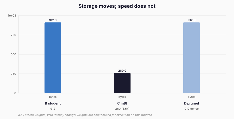
Figure 1. Stored bytes per student: 912, 260, 912. Latency identical to four decimals; accuracy retained at 0.997 of the weak baseline. Frozen E1 measurements.
The study uses RM-125, VERIFIED_PERMITTED for
train_compression_demo_e1. The compression pipeline is: train
(RM-125) → quantise/prune (same action, same record, no new
teacher, data, or outputs) → evaluate. The compressed artefact
inherits the base model’s rights position — under terms like
Gemma’s (L-004), a quantised student distilled from a restricted
teacher is still that teacher’s derivative, and a pruned copy is no
less derived for
having fewer weights. Here everything is self-created under the
repository’s terms, so the chain is clean by construction; the
L-004/L-005 context (Gemma derivative treatment, Llama naming and
scale conditions) is recorded for the regime where it would not be.
RM-104 and all prior records are untouched.
Limitations
One synthetic spiral, three seeds, tiny MLPs, and a deliberately weak student (budget noted above — the retention arithmetic is honest at the floor, not informative about ceiling behaviour). Single int8 symmetric per-tensor quantisation; no activation quantisation, no calibration set beyond weight statistics, no QAT. Single 50% pruning point, no retraining, dense execution only — no int8 or sparse kernel was benchmarked, by design. The D≥B ordering sits inside seed noise; no pruning benefit is claimed. No external replication and no independent review.
Preparing for evaluation
Part VI so far: choose by measured cost (Chapter 31), train cheaply where you can (Chapter 32), compress what remains (this chapter). Each step kept its own ledger and refused the others’ credit. What is missing is the audit that reads all three ledgers together: whether the correctness numbers mean what they claim, what the error bars hide, which slices fail while the average passes, and when a benchmark’s contamination voids the comparison. Chapter 34 builds that audit — and the first entry in it is this chapter’s own weak student, reported at 0.327 with the budget that explains it, rather than tuned into a success the protocol never authorised.
References
Sanh, V., Debut, L., Chaumond, J. and Wolf, T. (2019). DistilBERT, a distilled version of BERT: smaller, faster, cheaper and lighter. NeurIPS 2019 Workshop on Energy Efficient Machine Learning and Cognitive Computing (EMC2). arXiv:1910.01108. https://arxiv.org/abs/1910.01108
Jacob, B., Kligys, S., Chen, B., Zhu, M., Tang, M., Howard, A., Adam, H. and Kalenichenko, D. (2018). Quantization and Training of Neural Networks for Efficient Integer-Arithmetic-Only Inference. Proceedings of the IEEE/CVF Conference on Computer Vision and Pattern Recognition (CVPR). arXiv:1712.05877. https://arxiv.org/abs/1712.05877
Han, S., Mao, H. and Dally, W. J. (2016). Deep Compression: Compressing Deep Neural Networks with Pruning, Trained Quantization and Huffman Coding. International Conference on Learning Representations (ICLR, oral). arXiv:1510.00149. https://arxiv.org/abs/1510.00149
Leviathan, Y., Kalman, M. and Matias, Y. (2023). Fast Inference from Transformers via Speculative Decoding. Proceedings of the 38th International Conference on Machine Learning (ICML, oral). arXiv:2211.17192. https://arxiv.org/abs/2211.17192
Legal sources
Google Gemma Terms of Use. Last modified 1 April 2026. https://ai.google.dev/gemma/terms (retrieved 12 November 2026). Cited as L-004 for the derivative-works treatment of compressed or distilled derivatives; not legal advice.
Llama 3.2 Community License Agreement. Version released 25 September 2024. https://www.llama.com/llama3_2/license/ (retrieved 12 November 2026). Cited as L-005 for the naming, notice, and redistribution conditions context for compressed derivatives; not legal advice.