Distillation for Generative Media
Can a generative student produce useful samples with fewer inference steps than its teacher? Progressive halving on a 2-D mixture, a naive-striding baseline, and a null result: on this toy, step reduction costs nothing and distillation adds nothing.
Every chapter so far distilled a decision: a label, a ranking, a JSON document, an action, a fact from a store. This chapter distils a distribution. A diffusion teacher does not know the answer to any query; it knows how to turn noise into samples, one small denoising step at a time — dozens or hundreds of them. The student question is different from everything before it: not “can you be right more cheaply” but “can you draw from the same distribution in fewer steps, and what is lost when you do?”
Can a generative student produce useful samples with fewer inference steps than its teacher, and what quality, diversity, or stability is sacrificed?
On our bounded demonstration, the measured answer is a clean null with a positive latency ordering. Teacher (32 steps), distilled 16-step and 8-step students, and a naive 8-step strided teacher all land within noise of each other on sample quality (MMD 0.101–0.102) with full mode coverage everywhere; sampling time halves with each halving (0.026 → 0.012 → 0.006 seconds per thousand samples); the distilled 8-step student ties the naive 8-step baseline (0.1019 vs 0.1022). Step reduction costs nothing measurable here, and distillation adds nothing over naive skipping. Both halves of that sentence are findings about the toy, not about image models — and the chapter keeps them there.
Why diffusion sampling is expensive
A denoising diffusion model defines a forward corruption process and learns its reversal. The forward process adds Gaussian noise on a fixed schedule: with \(\bar\alpha_t\) the cumulative signal kept at step \(t\),
Noise prediction is a choice, not a necessity: predicting the clean sample \(\hat x_0\) or the score \(\nabla_{x_t}\log p_t(x_t)\) parameterises the same reversal (they differ by the known Gaussian algebra, \(\varepsilon = (x_t - \sqrt{\bar\alpha_t}\,x_0)/\sqrt{1-\bar\alpha_t}\)), and the demo predicts noise because the DDPM loss is then a plain mean-squared error, \(L = \mathbb{E}\lVert\varepsilon_\theta(x_t,t) - \varepsilon\rVert^2\), with no weighting to tune. The training objective is a simplified variational bound with the weights dropped — the standard DDPM simplification, stated as such rather than derived, since the demo needs the loss to work, not the bound to be tight.
One schedule disclosure, because schedules silently set task difficulty. The demo uses 32 linear steps from \(\beta_1 = 10^{-4}\) to \(\beta_{32} = 0.02\), so \(\bar\alpha_{32} \approx 0.72\): the forward process never reaches pure noise, yet sampling starts from \(N(0, I)\) regardless. That train-sample mismatch is a bounds-of-the-demo approximation — it works here (coverage 1.00 everywhere) and would need retuning, typically a cosine schedule with more steps, for any target where the last noise levels matter. A reader who ports the runner to 256 steps on harder data and keeps the linear schedule has changed the experiment; the manifest records the schedule so the change is visible.
Our target is deliberately minimal: a balanced mixture of four Gaussians at \((\pm3,\pm3)\) with \(\sigma = 0.5\) in the plane. Two dimensions, four modes, no pixels, no audio, no human judgement of quality. The chapter states this limit first because everything else — metrics, baselines, rights — follows from it. A demonstration that cannot fail on perceptual quality (there is nothing to perceive) can still fail on distribution quality, and does so measurably when a method drops a mode.
The progressive objective, halved
Progressive distillation (Salimans and Ho, P-034) turns a \(2N\)-step sampler into an \(N\)-step sampler, then repeats. The student initialises from the teacher and trains on the teacher’s own behaviour: from a noisy point \(x_t\), the teacher takes two deterministic DDIM steps (\(t \to t-1 \to t-2\)) while the student takes one (\(t \to t-2\)), and the student minimises
A stochastic sampler (DDPM ancestral sampling, or DDIM with \(\eta > 0\)) would make the same \(x_t\) branch into many \(x_s\), and regressing onto one draw would teach the student the noise of the draw as well as the direction of the denoising. The demo’s grids nest exactly (every student landing is two teacher steps down, asserted before training), which is what lets a single MSE compare them — stride against stride, no interpolation. The chapter derives it rather than asserting it because the derivation exposes the approximations: the student matches the teacher’s trajectory points, not the teacher’s distribution, and matching points implies matching distributions only insofar as the sampler visits them. Two samplers can agree on every training trajectory and disagree on coverage — the mode coverage metric exists to catch exactly that divergence.
Our demo applies the halving twice in sequence (32→16, then 16→8), each stage with 1,000 updates, each student initialised from its teacher. It differs from the paper’s procedure in one disclosed simplification: the paper iterates to convergence per stage on large image models; we run fixed small budgets on 2-D points. The mechanism — stride doubling by trajectory regression — is the same; the scale, the data, and the convergence story are not, and no CIFAR-10 or ImageNet number from that paper is cited as evidence here.
    flowchart LR
  T32[teacher: 32 DDIM steps] -->|regress 2-step targets| S16[student: 16 steps]
  S16 -->|regress 2-step targets| S8[student: 8 steps]
  T32 -.->|stride every 4th grid point| N8[naive 8-step baseline]
Figure 1. Each halving doubles the stride by regressing the teacher’s two-step result; the naive arm skips training entirely. The comparison that matters is distilled versus skipped, not versus the teacher.
Consistency and distribution matching, distinguished
Two alternatives the demo does not implement, distinguished so the reader does not confuse them with it. Consistency-style learning (Luo et al., P-035, a preprint) trains a model to map any point on the probability-flow trajectory directly to its origin — one evaluation from noise to sample, no stepping at all — by viewing guided reverse diffusion as an ODE to solve rather than a chain to walk; distilled from classifier-free guided diffusion teachers, a few-step latent consistency model reaches high-resolution images in 2–4 steps after tens of GPU hours, per the authors’ report (32 A100 hours for a 768×768 model — their figure, background only, not reproduced and not needed here).
Distribution-matching distillation (Yin et al., P-036) skips trajectories entirely: it matches the one-step generator to the teacher at distribution level, minimising an approximate KL whose gradient is a difference of two score functions (one of the target distribution, one of the generator’s), plus a regression term on large-scale structure — reaching, per the authors’ report, 2.62 FID on ImageNet 64×64 and comparability with Stable Diffusion at 20 FPS (their figures, background only). The three methods optimise different objects: trajectory points (progressive, ours), trajectory origins (consistency), distributions (DMD). The chapter implements the first at toy scale and describes the other two at background level, with venues and preprint status labelled — P-034 peer-reviewed at ICLR 2022, P-036 at CVPR 2024, P-035 a preprint — because choosing among them for a real system requires the compute, data, and metrics this book does not spend.
Example A — the tiny diffusion model
The teacher is a 3→64→64→2 MLP: two input coordinates plus a scalar time, SiLU activations, one noise vector out. It trains 1,500 updates on 2,000 mixture points with the DDPM noise-prediction loss. Sampling is deterministic DDIM from Gaussian noise down a fixed grid — 32 steps for the teacher, 16 and 8 for the students, 8 strided steps for the naive baseline (the teacher’s weights run on every fourth grid point, no distillation). Everything runs on CPU in seconds; the whole study fits in a 900-second ceiling with margin to spare (731 seconds wall time, not profiled by component; the measured sampling latency is a fraction of a second per seed, so sampling is not where most of it went).
Example B — the step-reduction comparison, per seed. Thirty-two teacher steps cost 0.022–0.030 seconds per thousand samples; sixteen cost 0.012; eight cost 0.006–0.007 whether distilled or strided. The latency halves with the step count almost exactly — the expected E3-style ordering (compute follows the loop count), measured. The quality ordering does not follow: MMD 0.0969/0.0966/0.0961/0.0964 (seed 100), 0.1057/0.1026/0.1053/0.1056 (seed 101), 0.1022/0.1033/0.1043/0.1047 (seed 102) for teacher/S16/S8/naive. Aggregates 0.1016/0.1008/0.1019/0.1022 — a spread of 0.0014 against per-arm standard deviations near 0.005. Nothing is distinguishable from anything; the honest aggregate table is four identical rows.
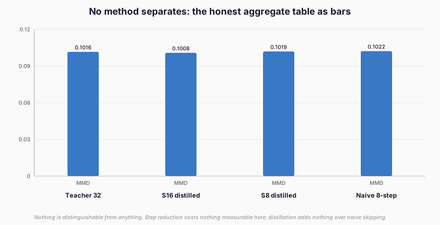
Figure 2. Mean MMD per arm with the per-seed spread implied: nothing beats noise. Frozen D30 measurements, descriptive.
The latency ordering tells the other half. Sampling 1,000 points costs roughly 0.026, 0.012, and 0.006 seconds at 32, 16, and 8 steps — halved each time, distilled or naive:
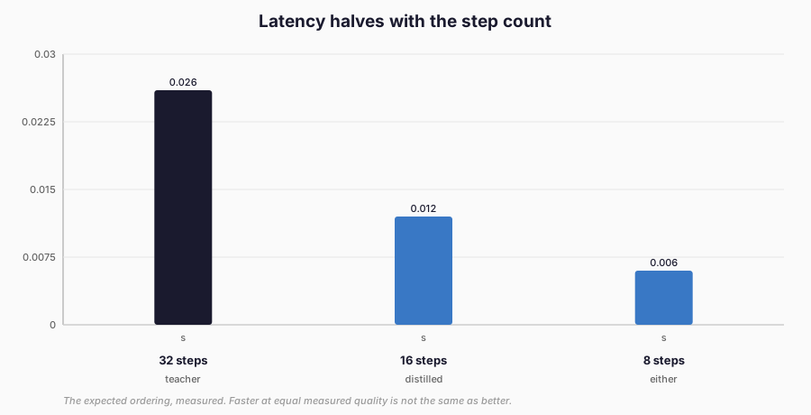
Figure 3. Seconds per thousand samples on CPU: the expected halving, measured. Faster at equal measured quality is not better. The per-seed winners rotate — S8 lowest on seed 100, S16 on 101, the teacher on 102 — which is the signature of noise, not of any method: a real effect would repeat its direction, and none does.
Sample quality, diversity, and what MMD cannot see
The primary metric is maximum mean discrepancy with an RBF kernel at the median-heuristic bandwidth, biased V-statistic, between 1,000 generated samples and 1,000 held-out reference points. MMD is deterministic given the samples, requires no density estimate, and is zero for identical sets — the test suite pins all three properties. Its blindness is stated alongside: MMD with one bandwidth cannot distinguish a mode dropped from a mode shifted by less than the bandwidth, and a single number never diagnoses which failure occurred.
That is why the chapter pairs it with mode coverage: each sample votes for its nearest mode, and the metric is the fraction of the four modes receiving at least 5% of samples. Coverage is 1.00 for every method on every seed, with per-mode fractions near 0.25 each — no collapse anywhere, including the naive baseline, which is itself informative: strided DDIM on this mixture loses nothing, so the task cannot separate careful distillation from careless skipping.
Diversity beyond coverage is reported as per-mode fractions rather than claimed: S8’s seed-100 split (0.23/0.25/0.24/0.28) is typical, and no arm concentrates or vacates a mode. Within-mode spread is not measured — the mixture components are isotropic Gaussians by construction, and asserting their preservation would need a finer-grained statistic the protocol does not run. Inadequate metrics are a failure mode the contract names, and this paragraph is the chapter practising the response: state what each number rules out, and name the ruling-out it cannot do.
Approximation error — the held-out one-step MSE of student steps against teacher two-steps — sits near 1e-9 (stage one) and 2e-8 (stage two): the students match the teacher’s jumps essentially exactly. That precision is suspicious in the productive way: it says the regression problem is trivial at this scale (the student initialises from the teacher and the targets are smooth), which explains why distillation ties naive striding rather than beating it.
When the student can copy the teacher’s steps exactly, and the naive baseline can skip them without penalty, there is no room for a method to demonstrate superiority. The demo is well-constructed for teaching and ill-constructed for ranking methods — which is why the chapter draws the teaching conclusion and refuses the ranking one.
What makes this not classifier distillation
Every earlier distillation in this book matched a discriminative signal: logits, relations, rankings, actions, facts. The teacher asserted something about an input, and the student learned to assert it more cheaply. A diffusion teacher asserts nothing. Its knowledge is procedural through and through: given noise at level \(t\), which direction is less noisy. There is no label to match, no class to agree on, no accuracy to report — the metrics of Chapters 5 through 29 do not type-check here, and importing them would be a category error rather than a reuse.
What transfers instead is a vector field over the input space (the denoiser’s output at each noise level), and the student is evaluated the way a sampler is evaluated: by the distribution of its outputs, not by any per-input decision. That is why the chapter’s mathematics (forward schedules, DDIM steps, trajectory regression) shares no symbols with the KL objectives of Part I, and why the rights analysis changes shape too: the risk is not a wrong label reproduced but a style, likeness, or voice reproduced — copying the distribution means copying what the distribution contains.
Why fewer steps do not imply a better model
The latency ordering (E3 in the evidence standard: supported — 0.026 → 0.012 → 0.006 s) tempts the inference the chapter refuses: if 8 steps match 32 on every measured axis, the 8-step model is “better”. It is cheaper at equal measured quality, which is a narrower claim with three explicit residuals. First, unmeasured axes: perceptual quality, fine detail, rare modes, and prompt-conditioned behaviour do not exist in this study, and the equality holds only where it was checked.
Second, stability: three seeds agree here, but step-skipping is known to diverge on harder distributions, and the demo’s stability does not transfer to them. Third, the teacher’s 32 steps are themselves arbitrary — a 64-step teacher might reveal differences the 32-step one cannot show, in either direction. “Faster at equal measured quality on this toy” is the complete claim; “better” would need the axes, the seeds, and the teacher the study does not have.
Failure modes, honestly listed
Treating diffusion distillation as classifier KD: the distilled object here is a sampler, not a classifier — no labels, no accuracy, no agreement metric would even type-check (see the preceding section). Mode collapse: the contract’s central fear, measured absent (coverage 1.00 everywhere, per-mode fractions balanced near 0.25 each); a collapse would read as coverage 0.25 with one mode holding nearly all samples, and the chapter reports the absence as a property of this toy, not as robustness of the method — a student that dropped a mode gradually (say, 0.15/0.30/0.30/0.25) would still score 1.00 coverage while misrepresenting the distribution, which is exactly why MMD accompanies it. Style and likeness appropriation: no images of anyone exist in this study, so the failure mode is untestable here — and that is precisely why it gets a scenario instead of a measurement (below).
A voice-cloning analogue sharpens the point: a distilled few-step voice model that preserves speaker identity has transferred the biometric, and no MMD-to-reference number settles whether that transfer was permitted. Inadequate metrics: MMD-plus-coverage is stated with its blindness (single bandwidth, no within-mode spread, no perceptual axis); FID would add a feature-space perceptual axis at the price of a pretrained Inception network the demo refuses to download — stated as a trade-off, not an oversight. Compute runaway: bounded by the 900-second ceiling and the tiny-model discipline; the study used 731 seconds (not profiled by component), and a larger demo would need its own authorisation. Claiming production quality from a toy demo: refused throughout — no FID, no human judgement, no comparison with any published image result.
A style and likeness scenario
Suppose the target were not four Gaussians but portraits in the style of a living illustrator, and the teacher a model trained on her work. The distilled student inherits the question, not just the weights: was the training data licensed for this use, does the teacher’s licence permit distillation into a competing generator, and does the student’s output appropriate a protected style or a recognisable likeness? The three questions separate. Training-data licence governs the teacher’s existence: scraped portfolios, opt-out registries, and text-and-data-mining reservations (the Chapter 37 register) decide whether the teacher should have been trained at all, and a distilled student does not launder an unlicensed teacher. Teacher terms govern the distillation act itself: Gemma-style derivative clauses and Llama-style naming and scale conditions attach at the moment of transfer, and the student inherits the stricter set.
Output rights govern deployment: style sits in the hardest part of copyright’s idea/expression terrain, while voice and likeness add personality-rights regimes that vary by jurisdiction and attach to recognisability, not to training method. A public portfolio is not a training licence; a model card’s permissive tag is not a complete rights analysis. This study answers none of those questions — it has no style, no likeness, no human data — and the scenario exists to mark where the engineering chapters end and Chapters 37 and 38 begin. The operative rule for the book’s own work: train only on data whose licence you have recorded for the specific act (here: self-created points, RM-122, no redistribution), and flag everything else for specialist review rather than resolving it by assertion.
Cost, stability, and rights
Teacher training costs ~1.4 seconds per seed (1,500 updates); each distillation stage ~1 second (1,000 updates); the naive baseline costs nothing beyond the teacher. The per-seed structure is identical — teacher, then stage one, then stage two, then four sampling runs — so the 731-second total divides evenly and the ceiling check is per-seed meaningful, not just a batch aggregate: no seed came within a factor of two of the 900-second budget. The wall time was not profiled by component, and the measured sampling latency is too small to account for it, so where the time went remains unmeasured.
Sampling latency per method is small (1,000 samples × up to 32 steps
on CPU); where the rest of the wall time went was not profiled.
Stability across seeds is exact in structure — coverage 1.00 nine
times out of nine, latency ordering identical — with MMD seed spread
(±0.004–0.005) exceeding every arm gap, which is why the chapter
reports aggregates with standard deviations and refuses rankings.
The study uses RM-122, VERIFIED_PERMITTED for
train_diffusion_demo_d30. The model-terms context (L-004’s
derivative/distribution conditions, L-005’s naming and notice
conditions) is recorded for the regime where a real teacher’s terms
would govern the distilled student; here the teacher is
self-created, so there is nothing to inherit, and the record says so
rather than assuming it. RM-104 and all prior records are untouched.
Limitations
A 2-D mixture; no images, audio, perceptual metrics, FID, or human judgement. One schedule, one denoiser size, one halving path, one naive baseline — no strided-16 intermediate, no learned-step-count variant, no second noise family. MMD at one bandwidth; coverage at one threshold; no within-mode spread. The step-reduction costs nothing measurable and distillation ties naive striding — the task is too easy to separate methods, stated as the reason no method is recommended. A harder target (overlapping modes, heavier tails, higher dimension) might separate them in either direction; the chapter does not predict which. Trajectory matching only; consistency and distribution-matching objectives are background. No external replication and no independent review.
Preparing for measurement
Part V moved the supervision signal across systems: rankings, structured outputs, actions, memories, experts, modalities, and now sampling trajectories. Every transfer was measured against an independent check — relevance labels, an integer evaluator, episode success, fresh vs stale queries, routing accuracy, cross-modal matching, reference-set MMD — and every chapter kept the check separate from teacher agreement.
Part VI turns the lens around: choosing the student (Chapter 31), shrinking the update (Chapter 32), compressing the weights (Chapter 33), and then the consolidated evaluation discipline (Chapter 34) that audits all of it. The demos get smaller and the measurements get stricter — which is the right direction, because the claims are about to get bigger, and Part VI supplies the student-selection, efficiency, and evaluation machinery those claims will be audited against.
References
Salimans, T. and Ho, J. (2022). Progressive Distillation for Fast Sampling of Diffusion Models. International Conference on Learning Representations (ICLR). arXiv:2202.00512. https://arxiv.org/abs/2202.00512
Luo, S., Tan, Y., Huang, L., Li, J. and Zhao, H. (2023). Latent Consistency Models: Synthesizing High-Resolution Images with Few-Step Inference. arXiv preprint. arXiv:2310.04378. https://arxiv.org/abs/2310.04378
Yin, T., Gharbi, M., Zhang, R., Shechtman, E., Durand, F., Freeman, W. T. and Park, T. (2024). One-step Diffusion with Distribution Matching Distillation. Proceedings of the IEEE/CVF Conference on Computer Vision and Pattern Recognition (CVPR). arXiv:2311.18828. https://arxiv.org/abs/2311.18828
Legal sources
Google Gemma Terms of Use. Last modified 1 April 2026. https://ai.google.dev/gemma/terms (retrieved 12 November 2026). Cited as L-004 for the Model Derivative and distribution-conditions context for distilling a generative teacher; not legal advice.
Llama 3.2 Community License Agreement. Version released 25 September 2024. https://www.llama.com/llama3_2/license/ (retrieved 12 November 2026). Cited as L-005 for the naming, notice, acceptable-use, and scale conditions context for derivative generation; not legal advice.