What Fine-Tuning Actually Changes
Trace a real CPU parameter update, separate context from learned state, and inspect a frozen base with a trainable adaptation branch.
Imagine a support team that wants a model to turn an incident report into a category, a severity and a routing decision. In this scenario, the current model often understands the report but returns an explanation where the downstream system expects a structured record. Sometimes it also chooses yesterday’s escalation route. The team proposes fine-tuning it on examples of the desired answers.
There are already two different problems in that proposal. Consistently following an output convention is a behavioural requirement. Knowing today’s escalation route requires access to the current policy. Training might help the first, while a policy lookup might serve the second more reliably. Neither possibility can be established by successfully running a training script.
Before choosing an intervention, we need a precise account of what it changes. Adding an example to a prompt changes the model’s input. Training changes stored numerical parameters. Training an adapter can change the combined model’s behaviour while leaving every original model parameter untouched. Distillation changes a student’s parameters using supervision supplied by a teacher. These statements describe different aspects of a system, and several can be true at once.
This chapter makes those distinctions observable. We will update a model small enough to calculate by hand, inspect every parameter, freeze the original transformation, train an added component, and reload the saved states. The experiment uses PyTorch on a CPU and downloads nothing. It establishes the mechanics on which later language-model experiments depend; it does not establish that a ticket-triage model has improved.
A model is a function with stored choices
Write a model as
Suppose the weights stay fixed and we supply a different incident report. The output changes because \(x\) changes. The intermediate numerical values computed for that report also change. Those values are activations: the results of applying the current operations to the current input. They are not newly learned weights. Retaining an activation in an inference cache changes what work a later computation can reuse; it does not, by itself, perform a parameter update.
For a language model, the context includes the tokenised instructions, examples, conversation and retrieved passages available to that invocation. A sentence placed in context can alter the response without becoming part of the parameters. The model may infer a useful pattern from examples in context, but ordinary prompting does not persist that pattern as a new weight update. Remove the examples and the input conditions have changed again.
Training introduces additional state. Gradients describe how the current loss changes with a parameter. Optimiser state is information an update rule retains across steps, such as momentum or running estimates of gradient moments. Parameters, gradients and optimiser state are distinct objects. Inference normally needs the parameters and the relevant execution configuration; reproducing a training continuation may also require optimiser state, scheduler state and random-number state. A saved set of model parameters is therefore not automatically a complete resumable training checkpoint.
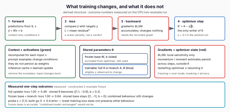
The figure maps the four operations onto the three kinds of state they touch: context and activations are recomputed per input, stored parameters divide into frozen and trainable sets, and gradients with optimiser state exist only to serve the next update. The outcome strip reports the chapter’s measured one-step CPU results on the constructed two-example fixture.
What the starting checkpoint already contains
Pretraining produces a starting parameter set by optimising an objective over a training corpus. For an autoregressive language model, a common objective rewards assigning probability to the next token given preceding tokens. Repeated updates can establish representations and capabilities useful beyond the original examples. They do not constitute a guarantee that any particular fact, instruction or operational policy will be handled correctly.
Fine-tuning starts from an existing parameter set and performs further training. Continued pretraining continues a corpus-level learning objective, often on a selected domain. Supervised fine-tuning, or SFT, uses examples of the desired behaviour, such as an incident report paired with the response we want the model to produce. With language models, those responses are usually sequences of target tokens; later chapters will examine exactly which tokens contribute to the loss.
The distinction concerns the starting point, data and objective. There is no special physical kind of “fine-tuning weight”. The numerical machinery still computes an output, evaluates an objective and updates permitted parameters. A checkpoint already adapted to instructions may undergo another SFT stage. A pretrained checkpoint may instead receive an adapter, preserving the original parameter values in storage while learning an additional transformation.
The progression can be drawn without assuming that every project needs every stage:
initial parameters -> pretraining -> starting checkpoint
                                      |
                    +-----------------+------------------+
                    |                                    |
            update selected original              freeze original parameters,
            parameters                            add trainable parameters
                    |                                    |
                    +--------------+---------------------+
                                   |
                          evaluate combined behaviour
This diagram tracks which parameters training can change. The supervision could come from demonstrations, preferences or a teacher. It also leaves out a valid engineering outcome: keeping the checkpoint unchanged and solving the task through its inputs or surrounding software.
One update we can account for completely
Consider a scalar output and a two-component input. Begin with
| Input \(x\) | Desired output \(y\) | Initial prediction \(\hat y\) | Residual \(\hat y-y\) |
|---|---|---|---|
| \((1,0)\) | 2 | 1 | −1 |
| \((0,1)\) | 0 | −1 | −1 |
The targets are constructed numbers, not labels from a real incident dataset. Define the loss as the mean squared residual over these two examples:
To improve this objective locally, we need its derivatives. A derivative tells us the change in loss per small change in a parameter, holding the other quantities fixed. Differentiating the squared residual and applying the chain rule gives
The learning rate is part of this account. The gradient is a local statement about the objective; it does not promise that an arbitrarily large step will improve it. Nor does this one improvement establish that more steps, a different objective or different examples would be useful. Those are questions an experiment must answer.
Forward, loss, backward, step
The update has four operations with separate responsibilities. The forward pass computes predictions using the current parameters. The loss calculation compares those predictions with targets under a chosen objective. The backward pass computes derivatives through the operations that produced the loss. The optimiser step uses those derivatives to change parameters.
In PyTorch, backward() accumulates gradients; it does not itself perform the SGD update. Clear old gradients when beginning a fresh step, or accumulation may change the update you intended. PyTorch’s versioned autograd mechanics describes how the operation graph supports differentiation. Our tests separately inspect values after the forward and backward passes and confirm that this model’s parameters change only when the optimiser steps.
This complete fragment reproduces the full-update calculation:
import torch

x = torch.tensor([[1., 0.], [0., 1.]], dtype=torch.float64)
y = torch.tensor([[2.], [0.]], dtype=torch.float64)
W = torch.nn.Parameter(torch.tensor([[1., -1.]], dtype=torch.float64))
b = torch.nn.Parameter(torch.tensor([0.], dtype=torch.float64))
optimizer = torch.optim.SGD([W, b], lr=0.1)

optimizer.zero_grad(set_to_none=True)
prediction = x @ W.T + b
loss = ((prediction - y) ** 2).mean()
loss.backward()
optimizer.step()

with torch.no_grad():
    print(W, b)
    print(x @ W.T + b)
The mathematical derivation treats each \(x\) as a column vector. The code stores examples as rows of a batch, so its matrix operation is x @ W.T. These are two layouts of the same calculation. Double precision makes the small arithmetic easy to inspect; it is not a prescription for efficient language-model training.
Full-parameter fine-tuning makes all original model parameters eligible for optimisation. That does not mean every scalar must change on every step. A particular gradient may be zero, a parameter may not participate in a computation, or an update rule may behave differently from this simple SGD step. “Eligible to change” and “observed to change” are distinct claims. Here the audit confirms that both weight entries and the bias changed by the amounts calculated above.
A frozen base can still be part of a changing model
Now preserve \(W\) and \(b\), and add a second branch:
The original LoRA paper applies a scaled low-rank update to selected transformations while freezing the pretrained weights. Our example uses scale one, no dropout and a single affine transformation. It is an educational analogue, not a complete LoRA implementation. In particular, a one-row matrix already has rank at most one: this miniature example demonstrates factorisation and freezing, not a meaningful compression advantage. Its adaptation branch has three trainable scalars, the same number as the original affine model.
Choose
After the recorded single step,
The implementation sets the base parameters’ requires_grad flags to false and excludes them from the optimiser. It then checks actual before/after values, as well as the absence of base gradients. Freezing is a training policy, not write protection: an explicit in-place assignment could still alter those tensors. A test deliberately introduces such a change to confirm that the audit detects it.
Freezing also differs from model.eval(), which selects evaluation behaviour for certain layers; it does not freeze their parameters. Conversely, disabling gradient recording around a whole adapted forward pass would prevent learning the branch. Later transformer examples must preserve the gradient paths needed by trainable components even when much of the model is frozen.
Running and interpreting the experiment
The executable implementation is examples/ch01/parameter_updates.py. Its snapshot and parameter_audit functions clone named parameter values and report gradients, trainability, deltas and norms. These are the first reusable instruments for FineTuneLab: before asking whether an adaptation helped, we can establish what it actually changed. They remain ordinary educational functions here; the full workbench is not yet implemented.
From the repository root, in a Python environment with PyTorch available, run:
python scripts/run_tests.py --output .local/ch01/my-test-timings.json
python -m examples.ch01.parameter_updates --output experiments/FT-01/my-run.json --checkpoint-dir .local/ch01/my-run
Choose new output paths for each run. The runner refuses to overwrite its report or checkpoint directory. It executes one step per model on the CPU using explicit starting tensors, seed 7, one computation thread, deterministic algorithms and float64. No random sampling is needed for these starting values. Seed control alone would not establish reproducibility; the tests also compare repeated numeric traces.
The original observed run is recorded in experiments/FT-01/run-001.json. The remediated implementation uses the declared learning rate and reproduces the same numerical results in experiments/FT-01-R1/run-001.json; the original evidence remains preserved. Rounded for readability, its results are:
| Quantity | Full update | Frozen base plus branch |
|---|---|---|
| Training loss before | 1.00 | 1.00 |
| Training loss after one step | 0.49 | 0.64 |
| Training predictions after | \((1.3,-0.7)\) | \((1.2,-0.8)\) |
| Stored base weight after | \((1.1,-0.9)\) | \((1,-1)\) |
| Stored base bias after | 0.2 | 0 |
| Reloaded predictions equal | Yes, bitwise | Yes, bitwise |
These are locally executed mechanism results, not a benchmark ranking of full fine-tuning and adapters. Their permitted changes differ, and the dataset and starting point were chosen to make the arithmetic transparent.
The input-only control evaluates the two inputs with an unchanged starting model: its outputs differ, but its stored parameters do not. That establishes the input/parameter distinction for this function. It is not an experiment on a language model’s ability to learn from a prompt.
Each trained model is saved as a state_dict and loaded into a fresh instance of its class using strict key matching. The check compares parameter names, shapes, dtypes, values, trainability flags and predictions; the new tensors must also have independent storage. The class constructor restores the freeze policy: state_dict is not relied on to encode requires_grad. The PyTorch saving/loading tutorial explains this separation between saved state and the model definition.
Both saved files contain the complete tiny model state. We have not built adapter-only packaging, a base-revision resolver or resumable optimiser checkpoints. The selected SGD has no momentum state, which makes this step easy to inspect but does not exercise the state required by more elaborate optimisers. The JSON preserves all input and parameter values, source hashes and checkpoint hashes; generated checkpoint binaries stay outside Git.
A lower loss can accompany a worse answer elsewhere
Consider another input, \(x=(1,1)\), with desired output zero. The original model predicts \(1-1=0\), so its squared error is zero. The fully updated model predicts \(1.1-0.9+0.2=0.4\). The adapted model predicts \(1-1+0.2(1+1)=0.4\). In exact arithmetic both now have squared error \(0.16\). The local run records floating-point approximations; \(0.4\) and \(0.16\) are rounded presentations of those recorded values.
The two training examples improved while this other behaviour deteriorated. Their gradients contained no requirement to preserve it. Shared parameters and shared transformations couple behaviours: adjusting a transformation for some inputs can change its outputs for others.
This probe was designed to expose interference. It is not a statistically representative test set, and the example is not evidence of the prevalence or magnitude of catastrophic forgetting in language models. It proves the narrower point that reducing one empirical objective does not logically guarantee preserving another. The later forgetting chapter will need actual capability probes and a controlled language-model experiment.
For incident triage, training loss is even further from the operational outcome. A token-level objective might improve while the model still emits invalid records, misses a severe incident, or follows an obsolete routing policy. We must measure the behaviours we require and the behaviours we need to preserve. Chapter 03 will specify that contract; Chapter 18 must freeze the benchmark and acceptance thresholds before real-model tuning.
The bridge to a language model
A transformer language model produces scores over possible next tokens. A common supervised objective is
The linear example’s squared error becomes a token objective; the forward computation becomes a sequence of interacting layers; differentiation follows many more paths. The logical roles stay recognisable: compute predictions, evaluate the objective, obtain gradients and update the permitted parameters. The learned result is a change in conditional probabilities. It need not contain a separately addressable rule corresponding to “always produce valid routing JSON”.
The miniature calculation omits attention, tokenisation, nonlinear representations, long sequences, mixed precision and the difference between training targets and sampled responses. It cannot show that an adapter has sufficient capacity for a task, that a model fits a particular GPU, or that training beats a prompt. Those are planned experiments, currently NOT_RUN for this book’s real-model path.
Preference optimisation changes the supervision and objective again. Instead of supplying only a desired answer, a dataset might identify which of two answers is preferred for the same input. DPO is one method for learning from such comparisons. Reinforcement learning approaches can optimise a reward signal, sometimes learned from preferences. These remain parameter-learning procedures; preferences do not make gradient descent disappear, and agreement with collected preferences does not establish universal correctness. The InstructGPT paper provides a concrete historical sequence of supervised demonstrations followed by preference-based training, rather than evidence that the same recipe will solve our task.
Prompting, retrieval and distillation occupy different axes
Prompting changes the context presented to the model. Retrieval can select current evidence to place in that context. Updating a document store need not update the generator’s weights. However, a retrieval-augmented system can also train its retriever or generator: the original RAG research explicitly investigated a trained retrieval-augmented model. Retrieval and fine-tuning can therefore be combined; their names do not describe mutually exclusive system designs.
Distillation describes a relationship between supervision and models. A teacher supplies outputs, distributions or other learning signals; a student is trained to reproduce selected aspects of that behaviour. The foundational distillation paper studies transferring predictive knowledge into a deployable model. If a student begins from an existing checkpoint and learns from teacher-produced responses, that process can be both distillation and supervised fine-tuning. The student may use full updates or adapters. It is misleading to contrast distillation with fine-tuning as though only one changes parameters.
These distinctions suggest useful questions about any proposed intervention. What changes at request time? Which persisted parameters can training modify? Where does the supervision come from? What information must remain current? What evidence would justify carrying the extra trained artefact into operation? An adapter answers the parameter question; it does not answer the others.
For the support team, a sensible next step might be a stronger prompt, deterministic schema validation, a current policy lookup, an adapter, or a combination. FineTuneLab must also be able to recommend a rule-based solution or no training. Chapter 02, When Fine-Tuning Beats Prompting, RAG, Tools or Distillation, will develop that choice. We can now approach it with a concrete distinction: changing the input changes the conditions of a computation; training changes the permitted numerical machinery used to perform it. Whether either change improves the system remains an evaluation question.
Exercise and implementation status
Before changing the script, calculate the full-update predictions for \(x=(1,1)\) at learning rate \(0.05\). Then predict the first gradient of \(A\) if both low-rank factors begin at zero. Check each claim in a new run or a small test without replacing the recorded experiment. Explain why a non-changing trainable parameter is not sufficient evidence that the optimiser is broken.
Status: TECHNICALLY_CHECKED_WITH_LIMITATIONS; author accepted with limitations; unpublished draft. The CPU update, parameter audit, finite-difference gradient check, frozen-base behaviour and save/reload checks have executed. This chapter demonstrates a mechanism on a constructed affine problem. No pretrained language-model adaptation, ticket-triage quality result or performance comparison is claimed. The author supplied an independent-review summary and accepted the chapter; remediation and its provenance are recorded in editorial/ch01-remediation-ledger.md. Verified source URLs and access dates are recorded in research/ch01/sources.md; the original experiment protocol and limitations are in research/ch01/README.md.
Further Reading
- Edward J. Hu et al., “LoRA: Low-Rank Adaptation of Large Language Models” (2021). Read the source. The original low-rank adapter paper behind the chapter’s frozen-base branch, including evidence on why low-rank updates can suffice.
- Geoffrey Hinton, Oriol Vinyals and Jeff Dean, “Distilling the Knowledge in a Neural Network” (2015). Read the source. The foundational distillation paper, showing how teacher supervision transfers behaviour into a deployable student model.
- PyTorch contributors, “Saving and Loading Models” (living documentation). Read the source. The authoritative reference for the chapter’s save/reload audit, separating parameter state from optimiser state and eval mode.