Optimisers, Learning Rates and Precision
Derive SGD and AdamW updates, preserve token-weighted accumulation, and inspect clipping and mixed precision with checked arithmetic.
A gradient of $-8$ is not a new weight. It is a local sensitivity: increasing the parameter slightly should reduce the current loss. An optimiser must decide how that sensitivity changes the parameter, how previous sensitivities matter, whether to shrink the weight, and when an update should happen. Two scripts can start with the same parameters and gradients yet follow different training paths because those decisions differ.
We will derive the updates separately from the Transformer, check their arithmetic against PyTorch, then apply the same rules to the model developed in Chapter 09. The reference calculations use float64 to expose numerical agreement. The shared training experiment uses FP32; a separate bounded CUDA probe investigates selected FP16 operations.
Take one controlled step
Gradient descent updates parameters by
The local approximation is $L(\theta+\Delta)\approx L(\theta)+g^\top\Delta$. Substituting $\Delta=-\eta g$ produces a negative first-order term, $-\eta\|g\|^2$, for positive $\eta$. Curvature supplies higher-order terms. A displacement that is too large can cross the region in which the local approximation was useful and increase the loss instead.
Stochastic and minibatch gradient descent use estimates of a larger data objective’s gradient. The particular examples, their target counts and the reduction convention all influence that estimate. A larger batch can reduce some sampling variation, but it does not repair biased labels or an unintended objective.
Carry a velocity, not just the latest gradient
A simple momentum convention is
For a weight initially 1, learning rate 0.1 and momentum 0.9, a first gradient 2 gives velocity 2 and weight 0.8. A next gradient 1 gives velocity 2.8 and weight 0.52. The second displacement still reflects the first gradient. The pure-Python reference and PyTorch’s tested SGD configuration agree under this convention.
This historical state explains why restarting an optimiser is not generally equivalent to continuing it. Restoring only the weights preserves the current function but loses the velocity that determines its next movement. Chapter 12 will distinguish an intentional new adaptation phase from an interrupted run that should continue the same update trajectory.
Derive Adam’s two running statistics
Adam maintains first- and second-moment estimates for each parameter element:
At the first update, if the scalar gradient is non-zero, the bias-corrected estimates equal that gradient and its square. Ignoring $\epsilon$, their ratio becomes its sign. That does not mean Adam permanently discards gradient magnitudes. Later moment histories, changing gradients and $\epsilon$ all influence the direction and scale.
AdamW adds decoupled weight decay:
Reproduce several updates, including their history
The reference starts from $[1,-2]$, uses learning rate 0.01, $\beta_1=0.9$, $\beta_2=0.999$, $\epsilon=10^{-8}$ and decay 0.1. Three supplied gradients produce:
| Step | Gradient | Updated first parameter | Updated second parameter |
|---|---|---|---|
| 1 | $[0.5,-0.25]$ | 0.989000000200 | -1.988000000400 |
| 2 | $[0,0.5]$ | 0.981310417848 | -1.989673035577 |
| 3 | $[-0.1,0]$ | 0.976504339517 | -1.990513353329 |
The independent scalar implementation and PyTorch float64 AdamW returned the same recorded values in the reference run. The first step can be checked directly: decay changes the first weight to 0.999, and its normalised gradient update is almost 0.01. The small departure from 0.989 comes from $\epsilon$.
A zero current gradient does not imply a zero displacement. Weight decay can still shrink the parameter, and non-zero moment history can still move it. A missing gradient buffer is different again. In the tested PyTorch configuration, a parameter whose gradient is None is skipped, whereas one with an explicitly zero gradient participates. Starting each at 1 with learning rate 0.1 and decay 0.1 moved the zero-gradient parameter to approximately 0.99 and left the missing-gradient parameter at 1.
These details are part of an optimiser interface, not assumptions to infer from a method’s name. The AdamW API records the available options. Our arithmetic comparisons explicitly use the ordinary non-foreach reference path and the pinned library version.
Accumulate the intended gradient
Suppose an optimiser step covers microbatches with selected-target counts $N_1,\ldots,N_M$. The desired token-mean gradient is
We check this with the original Chapter 07 batch, whose two rows have three and four targets. A full-batch backward calculation and correctly weighted accumulation differed by at most approximately $5.6\times10^{-17}$ in float64. Incorrectly averaging the two means produced a maximum parameter-gradient difference of approximately 0.04929. Both computations completed successfully; only one preserved the declared objective.
The reusable accumulate_token_mean function implements that denominator and is also called by the final training loop. It clears no gradients and performs no optimiser step: the caller controls the step boundary. The caller clears the buffers once, accumulates all microbatches, clips if desired, performs one update and advances the schedule once.
Accumulation is not universally equivalent to a larger physical batch. Dropout changes sampled masks; batch-dependent operations can change the forward function; floating-point reduction order can change rounding. Taking an optimiser step after each microbatch changes moment states and the parameters used by later microbatches. The equality check here fixes the model, disables dropout and compares the same token-weighted objective before any update.
Clip after accumulating and before updating
Global norm clipping replaces a gradient vector by
Clipping each microbatch independently is a different nonlinear operation from clipping their accumulated gradient. It can change the final direction as well as its magnitude. Our loop clips once after the complete accumulation. It rejects non-finite norms rather than allowing an infinite or NaN gradient to become a mysterious parameter failure several steps later.
Clipping limits a displacement component induced by large gradients; it cannot make an excessive learning rate safe in general. It also does not correct a wrong loss mask or restore information lost to low-precision arithmetic.
Make the learning-rate schedule an explicit part of the experiment
A schedule chooses $\eta_k$ as training progresses. Warm-up initially limits the step size; decay reduces it later. Neither is a substitute for defining which counter advances the schedule. Advancing after every microbatch instead of after every optimiser step changes a run with accumulation.
The bounded capstone uses a deliberately explicit multiplier, with step index $k$ starting at zero:
Changing the schedule, its total step count or its position changes the next update even with identical model and optimiser moment arrays. A resume checkpoint must therefore preserve its configuration and state. A new adaptation phase may intentionally use a fresh schedule, but should say so.
Separate storage, computation and scaling precision
FP32, FP16 and BF16 allocate their bits differently. A narrower representation can reduce storage and accelerate supported operations, but it changes range and rounding. BF16’s exponent range differs from FP16’s, while its fraction has fewer bits. A dtype name alone does not establish that a device executes it natively or that the chosen model path is compatible.
In the actual CUDA probe, a tensor constructed in FP16 from $10^{-8}$ became zero, and one constructed from $10^5$ became infinite. These are one-element numerical observations, not intentional memory failures. The main educational training remains FP32. BF16 was not requested on the reference RTX 2060.
The mixed-precision probe keeps parameters in FP32 and uses autocast for selected operations. Its logits were FP16 and its cross-entropy loss was FP32. There is no separate extra master-weight copy in that arrangement because the stored parameters already have FP32 precision. Other arrangements may maintain a distinct master copy and must count it.
Loss scaling multiplies the loss before backward and divides the resulting gradients before the update. In exact arithmetic this changes no intended gradient; in finite arithmetic it can keep small intermediate derivatives away from underflow. It cannot reconstruct distinctions lost in the forward pass or make an already infinite forward value meaningful.
The successful CUDA probe used the order:
scaler.scale(loss).backward()
scaler.unscale_(optimizer)
clip_grad_norm_(model.parameters(), 1.0, error_if_nonfinite=True)
scaler.step(optimizer)
scaler.update()
Clipping before unscaling would apply the bound to the scaled gradient and impose a different effective threshold. The observed scaler value remained 128 after this finite update. We do not claim to have demonstrated recovery from arbitrary overflow: this probe requires a finite unscaled gradient and aborts if that check fails. General mixed-precision methods are described in Mixed Precision Training; our evidence is this much smaller, explicitly bounded operation.
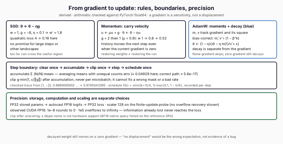
The three lanes show why the update rule is itself an experimental choice: the same gradient displaces the weights differently under SGD, momentum and AdamW. The strips below fix the step boundary that the surrounding sections warn about — accumulate with token weights, clip once, step and schedule once — and separate the precision observations from any claim of overflow recovery.
The optimiser now connects a checked gradient to a reproducible parameter update. Its state, rate schedule, accumulation convention and precision are all part of that connection. Chapter 11 measures the runtime consequences: which arrays exist, what the allocator retains and how much work an update actually performs.
Further Reading
- Diederik P. Kingma and Jimmy Ba, “Adam: A Method for Stochastic Optimization” (2014). Read the source. The optimiser paper whose moment updates and bias correction the chapter reimplements and checks against PyTorch.
- Ilya Loshchilov and Frank Hutter, “Decoupled Weight Decay Regularization” (2017). Read the source. Establishes the decoupled-decay distinction the chapter verifies in arithmetic, where decay still moves a zero-gradient parameter.
- Razvan Pascanu, Tomas Mikolov and Yoshua Bengio, “On the difficulty of training Recurrent Neural Networks” (2012). Read the source. The original gradient-clipping reference behind the clip-after-accumulation rule and its limits.