Budget the Adaptation
Account for adaptation memory and lifecycle cost, preserve unknown runtime quantities, and separate analytical feasibility from permission and measured training fit.
A model’s weight file looks comfortably smaller than the GPU’s memory capacity. The proposed training run nevertheless fails before its first useful update. Nothing about this is paradoxical. The file counted one representation of the parameters; training required other state, and some of the GPU’s memory was already occupied.
The opposite mistake is also possible. An engineer adds a universal number of bytes per parameter, concludes that adaptation cannot fit, and never investigates a frozen-base method that maintains training state for a much smaller parameter set. A useful budget needs the right accounting boundary, not merely a pessimistic constant.
Chapter 03, Write the Task Contract Before Training, defined the outcome an experiment must earn. This chapter budgets the resources and work needed to investigate it. We will calculate specified tensor storage, express implementation-dependent quantities as assumptions or ranges, inspect actual hardware without training, and build a resource assessment that can return insufficient evidence. An estimate may justify designing a bounded canary. It cannot substitute for one.
Begin with units and representations
Let \(P\) be the number of stored parameters and \(b\) their storage width in bits. Ignoring packing and metadata, the storage is
For a hypothetical 600-million-parameter model, 16-bit weights occupy 1,200,000,000 bytes. That is 1.2 decimal GB, about 1.118 GiB. A GB is \(10^9\) bytes; a GiB is \(2^{30}\). The distinction is large enough to matter near a memory limit. FineTuneLab requires explicit units for conversions and names quantities in bytes or MiB rather than using an ambiguous “G”.
Storage precision and computation precision are separate choices. A quantised base can be stored compactly while arithmetic uses a floating-point representation. An implementation may also retain another copy of parameters for updates. Selecting a computation dtype in a configuration does not establish that the GPU supports it natively, that a particular kernel exists for it, or that the trainer uses the representation the budget assumed.
The relevant inventory is the actual parameter collection, including any embeddings, output heads, biases and shared/tied representations. Do not multiply a file size by a guessed factor and treat the result as a measured training requirement. Nor should a model’s marketing size stand in for an inspected parameter count. Our example explicitly declares 600 million parameters; it does not identify a real checkpoint or infer its architecture.
Training introduces another parameter population
Write \(T\) for the number of trainable parameters. Full fine-tuning usually makes the original collection trainable, so \(T=P\). Partial fine-tuning may update a selected subset. A frozen-base adapter adds its own trainable tensors, which may not be part of the original \(P\).
Gradients consume storage associated with the trainable parameters. Optimisers may retain additional arrays. For a specified gradient width \(b_g\), \(k\) optimiser-state arrays of width \(b_o\), and an explicitly selected separate master copy of width \(b_m\), a simple ledger is
For the full-update illustration, choose FP16 stored weights, FP32 gradients, two FP32 optimiser-state arrays and a separate FP32 master copy. The ledger is then:
| Selected tensor population | Bytes |
|---|---|
| Base weights | 1,200,000,000 |
| Gradients | 2,400,000,000 |
| Two optimiser states | 4,800,000,000 |
| Separate master copy | 2,400,000,000 |
| Total before runtime memory | 10,800,000,000 |
This example has 18 bytes per original parameter under its chosen assumptions. It is not a claim that every trainer uses 18. The Transformers memory anatomy documentation provides a useful inventory of these categories; the ledger must still be checked against the selected runtime. We do not import its model-specific memory figures as results for this project.
Even the tensor total is not a full training budget. A run must also compute predictions, retain information for differentiation, perform updates, move data and preserve recovery artefacts.
Activations depend on the computation
Activations are the intermediate values produced for a particular batch. Some must remain available for backward computation. Their memory depends on the architecture, sequence length, microbatch, precision, gradient paths and kernels. A parameter count alone cannot determine it.
A straightforward attention implementation can materialise an object with a sequence-by-sequence dimension. That component scales quadratically with sequence length. Other retained tensors can scale linearly, and alternative kernels can change which objects are stored. Consequently, doubling a sequence may have a very different memory effect from doubling a small affine training dataset. The architecture and execution path matter.
Microbatch size controls how many examples participate in one forward/backward computation. Gradient accumulation can combine gradients across several such computations before an optimiser step. If the microbatch is \(B\) and the accumulation factor is \(G\), the nominal effective batch is \(BG\) examples, subject to details such as variable-length examples and loss normalisation. Accumulation does not require retaining \(G\) complete forward graphs in an ordinary loop that releases each graph after backward. It also does not promise identical optimisation or throughput to a physically larger batch.
Activation checkpointing trades retained values for recomputation. The PyTorch checkpoint documentation describes the mechanism. Its benefit depends on which computation is checkpointed and on the actual implementation. Our estimator therefore does not apply a universal percentage discount when a checkbox is enabled. A supplied activation profile must match its model identity, computation dtype and checkpointing setting.
For a transparent sensitivity exercise, we allow a caller to propose coefficient ranges in
Our fictional profile uses \(a\) between 262,144 and 524,288 bytes per token and \(q\) between zero and 128 bytes per token squared. At microbatch one and sequence length 512, this gives 128–288 MiB. At sequence length 1,024 it gives 256–640 MiB. At sequence length 512 and microbatch two it gives 256–576 MiB. Increasing accumulation alone leaves this activation envelope unchanged. These are executed arithmetic results on invented coefficients, not measurements of a 600-million-parameter transformer.
Missing coefficients produce UNKNOWN. A precise-looking value fabricated from model size would be less useful than an honest gap.
The allocator is not the tensor ledger
Runtime memory also includes temporary workspaces, CUDA context and library allocations, communication or update buffers, and allocator behaviour. A cached allocator can reserve memory beyond the bytes occupied by currently live tensors. Fragmentation and the timing of allocations can prevent a request from succeeding even when a sum of ideal payloads looks small. The PyTorch CUDA memory documentation distinguishes allocated tensor memory from memory managed by the caching allocator.
FineTuneLab accepts separate workspace and allocator-headroom ranges. They must cover the intended implementation boundary, including overhead not counted elsewhere. It does not infer a safe reserve from the GPU name. In the demonstration those ranges are fictional: 256–512 MiB for workspace and 512–1,024 MiB for allocator/headroom. Together with the activation envelope, they create a device-memory range under stated assumptions.
Two conclusions are possible without a measured peak. If known required payload alone exceeds the available budget, the proposal cannot fit that budget under those assumptions. If a complete assumed upper bound lies below the limit, the arithmetic is consistent with fitting. The second conclusion depends on the completeness and realism of the assumptions, while the first can remain valid even when other positive terms are unknown.
An unbounded term must not silently become zero. The report preserves unknown terms and withholds an upper bound. Its lower bound is the sum of known contributions only. Passing that lower bound beneath the limit is not evidence that the complete computation fits.
What adapters and quantisation change
For a linear transformation with input width \(d_{\mathrm{in}}\), output width \(d_{\mathrm{out}}\) and low-rank factors of rank \(r\), the two added matrices contain
Twelve selected 1,024-by-1,024 transformations at rank eight contain 196,608 adaptation parameters. This is the declared target set in our example, not a complete architecture inferred from “600M”. With FP16 adapter storage and the same specified gradient/state/master widths, adapter-associated tensors add 3,538,944 bytes. The frozen FP16 base still occupies 1.2 billion bytes. Lower training-state storage does not remove the forward computation or guarantee a proportional reduction in activations.
The comparison below reports selected persistent tensor payloads only:
On this estimator’s adapter path, all declared trainable components are stored separately alongside a fully frozen base. That can represent an added head or a saved trainable copy. Updating an existing bias or head in place needs a different storage ledger; the count alone does not tell us which copies exist. The present adapter layout does not model that hybrid in-place case.
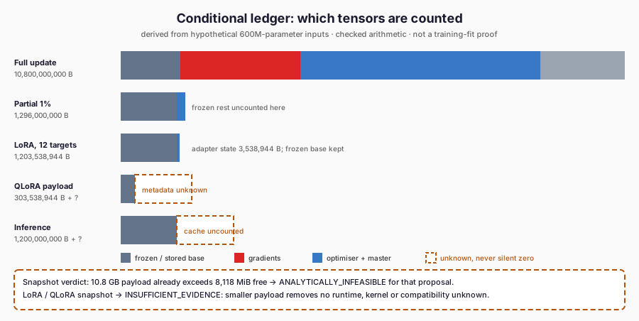
The bars show the same lesson as the table: the full-update payload is dominated by gradients and optimiser state, while the adapter proposals shrink the counted tensors but leave workspace, activations and allocator behaviour unknown. The verdict strip records what follows from the captured 8,118 MiB snapshot alone — rejection for the full proposal, insufficient evidence for the rest.
| Method and explicit assumption | Trainable count | Selected tensor bytes |
|---|---|---|
| Full update of hypothetical 600M base | 600,000,000 | 10,800,000,000 |
| Partial update of 1% of that base | 6,000,000 | 1,296,000,000 |
| LoRA on twelve declared matrices | 196,608 | 1,203,538,944 |
| QLoRA packed-base payload plus selected adapter state | 196,608 | 303,538,944, with quantisation metadata still unknown |
| FP16 inference weights, no training state | 0 | 1,200,000,000, with inference runtime/cache memory uncounted |
| Three-parameter FP32 CPU teaching model, no optimiser state | 3 | 24, including gradients; process/framework memory uncounted |
For QLoRA, the four-bit number concerns the frozen base representation. Trainable adapters, their gradients, optimiser state and possible master copies use their own representations. Quantisation scales, other metadata and kernel buffers are additional. The estimator’s 300-million-byte packed base is therefore a payload lower bound, not the complete base allocation or a full QLoRA memory budget.
The demonstration deliberately leaves QLoRA activation and metadata requirements unknown. It uses a shared fictional activation envelope for the full/partial/LoRA arithmetic exercise only to expose the accounting difference; that is not evidence that their real backward graphs retain identical memory. A real comparison needs separate measurements or defensible profiles for each implementation.
The inference case similarly lacks an execution/cache profile. A weight payload that fits says nothing about how many concurrent or long-context requests can be served, and it does not establish training fit.
Budget host RAM, recovery and storage separately
GPU memory is only one resource. Tokenisation and data preparation can consume host RAM. Loading a model can temporarily retain more than one representation. Offloading moves some pressure to host memory and transfer bandwidth; it does not make that state disappear. Worker processes, dataset caches and evaluation outputs can introduce further requirements.
Checkpoint storage depends on what is saved. An adapter-only artefact can be small but still depends on a compatible base elsewhere. A resumable training state can include optimiser and master state, while ordinary saved model parameters do not necessarily include either. Atomic replacement or retaining a recovery copy can temporarily require additional disk space. Dataset revisions, model caches, reports and multiple failed trials also remain on disk unless a retention policy removes them.
FineTuneLab computes a checkpoint-payload floor for the selected save scope and retained-copy count. It excludes file metadata, quantisation metadata and an externally stored base for adapters. A floor is not a file-size prediction. Host and disk requirements can be supplied as separate ranges and tested against explicit limits; otherwise their absence remains visible. The resource classification’s scope is device memory plus whichever host/disk/time limits the caller actually supplied. It is not a certificate that every lifecycle requirement has been measured.
Training time is likewise unknown without a supplied step-time assumption or measurement. The module can multiply a stated step-time range by a step count, but it cannot discover throughput from parameter count. A configuration can be admissible in memory and unacceptable in time, or the reverse.
The actual local GPU is a separate observation
A fresh read-only probe on 17 November 2026 reported an NVIDIA GeForce RTX 2060 with 12,288 MiB total memory and compute capability 7.5. The captured nvidia-smi observation showed 8,118 MiB free and 3,944 MiB used, with driver 591.44. These fields are recorded as reported; they need not sum to the total because driver accounting can include other categories. Free memory is a time-specific observation, not a fixed property or a promise about a later run.
The environment used Python 3.13.15, PyTorch 2.6.0+cu124 and a reported CUDA runtime build of 12.4. CUDA enumeration succeeded. Transformers metadata reported 5.17.0, while Datasets, PEFT, TRL, Accelerate and bitsandbytes were not installed. Package metadata presence does not establish that an end-to-end trainer imports and runs correctly.
PyTorch’s BF16 query returned true when emulation was included, but false for native support. The admission code rejects a request requiring native BF16 on this reported device. A dtype option exposed by a framework must not be mistaken for native hardware support.
The NVIDIA compatibility documentation explains driver/runtime compatibility boundaries and limitations. A newer driver number and successful device enumeration are useful facts; neither checks the chosen trainer, model or quantised kernel on native Windows. Our report keeps runtime training compatibility unknown. No model was loaded, no GPU tensor allocation was requested and no forward/backward canary was performed.
Under the selected full-update assumptions, 10.8 billion bytes of persistent tensor payload already exceed the captured 8,118 MiB free budget. The estimator can reject that proposal against that snapshot without inventing an activation measurement. This is not a measured out-of-memory event, nor a claim that every full update of every 600M model fails on a 12 GiB device. Changing implementation, precision, offloading, the available budget or the update strategy changes the proposal.
The LoRA and QLoRA snapshot comparisons return insufficient evidence. A smaller known payload does not erase missing runtime compatibility or quantisation/activation information. Chapter 05 will choose a candidate checkpoint; this chapter has not done so by hiding a model behind a parameter count.
Adaptation cost extends beyond the GPU bill
Dataset construction, annotation, review and synthetic generation can cost more than a short training run. Training attempts can fail, and useful experiments need controls and evaluation. Saved artefacts require storage. A deployed model needs monitoring, incident handling and maintenance; changing policy or labels can require another evaluation or release. These are part of the adaptation decision, not optional footnotes after a successful update.
We reuse Chapter 02’s break-even model. Let \(F\) be fixed incremental cost relative to an admissible baseline over a stated horizon, and let \(c_0\) and \(c_1\) be expected per-request costs. If \(c_0>c_1\), equality occurs at
Our fictional cost case has 1,000 units of annotation/review, 1,000 of training attempts, 500 of evaluation and 500 of maintenance: 3,000 total incremental units. Its two five-hour training attempts at 100 units per hour and full assumed utilisation account for the training term. Flat blended token rates and 1,000 tokens per request give 0.010 baseline units versus 0.004 candidate units. Equality is at 500,000 requests, just as in Chapter 02. These are hypothetical accounting inputs, not prices, measured training hours or demonstrated savings.
Sensitivity changes the conclusion without changing the algebra. At one million requests, the same assumptions give 3,000 units of net savings. Doubling candidate token usage moves break-even to 1.5 million requests; it is not enough to say that the candidate has a cheaper token rate. Doubling the assumed training attempts, halving utilisation under this billed-wall-time model, doubling label time, or increasing maintenance from one event to three each raises the fictional fixed total to 4,000 units. Break-even is then about 666,667 requests. Non-terminating decimal divisions are represented at a fixed 28-digit Decimal precision, rather than being presented as infinitely exact numbers.
The utilisation relationship is an assumption: the example bills useful training hours divided by utilisation. It is not a measured law relating GPU occupancy to training throughput. Similarly, a flat blended token rate is only a simplified cost input. Actual retry, output-length, retrieval and human-review costs must enter the relevant per-request boundary.
No monetary saving compensates automatically for a failed task contract. Latency and quality constraints remain separate. FineTuneLab’s cost report explicitly says they have not been evaluated. Its contract-aware admission path flags missing cost evidence or a fixed cost exceeding the declared training budget, while preserving the original contract hash.
Read the admission result carefully
The reusable module is ftlab.budget; lifecycle arithmetic is in ftlab.costing. Both are usable without PyTorch or a GPU. The proposal schema names total/trainable counts, low-rank dimensions, storage and computation dtypes, selected state arrays, sequence/microbatch/accumulation, checkpointing, optional memory profiles and resource limits. Unknown fields, invalid dtypes, negative counts, inconsistent ranks and impractically large inputs produce diagnostic codes. Nested assumption values are revalidated when consumed.
Resource assessment has four outcomes. ANALYTICALLY_FEASIBLE means the scoped calculation fits under supplied complete device-memory and compatibility assumptions. ANALYTICALLY_INFEASIBLE means a required lower bound exceeds a supplied limit. INSUFFICIENT_EVIDENCE preserves unknown quantities or a range crossing the limit. INCOMPATIBLE identifies a configuration such as unsupported native BF16 or unavailable CUDA.
A separate contract result can block a resource-feasible proposal. Our reference task still prohibits training at this stage, has unverified model rights, a zero training budget and unfrozen benchmark prerequisites. The fictional LoRA memory case therefore does not become an authorised experiment. Its report records the resource calculation and the contract blockers separately. Every path keeps training_verified=false; the component never launches anything, and launch_allowed remains false.
Run the complete example from the repository root:
New-Item -ItemType Directory -Force .local | Out-Null
python scripts/probe_environment.py | Set-Content -Encoding utf8 .local/ch04-hardware.json
python -m examples.ch04.budget_demo --hardware .local/ch04-hardware.json --output experiments/FT-04/my-run.json
python scripts/run_tests.py --output .local/ch04-test-timings.json
Choose new report paths and create the local output directory if needed. The probe reads software/device metadata; the demo then uses that captured observation without probing again. Its arithmetic can be reproduced against the saved hardware record even when today’s free memory has changed. The report distinguishes declared coefficients, computed bytes, observed hardware and unverified execution.
The cases include full and partial updates, LoRA, QLoRA with unknown overhead, inference, a tiny CPU teaching model, a four-GiB over-budget limit, unsupported precision, missing model metadata and sequence/batch sensitivity. Conditional examples assume runtime support explicitly; actual-snapshot cases keep it unknown. These are not measured comparisons between training libraries.
A canary is still required
Before a later real run, first resolve the rights, task, dataset, model revision and environment prerequisites. Then propose a bounded canary using the chosen checkpoint and actual input formatting. A possible initial protocol is microbatch one, a short fixed sequence, at most ten optimiser steps and at most 120 seconds including loading. These are proposed stop limits, not permission to run it or a prediction that it will finish. Any such long integration test must be explicitly scheduled and marked LONG rather than joining routine chapter checks.
Recheck available memory immediately beforehand. Record allocated and reserved peaks, process/runtime overhead, wall time, loss and parameter trainability. Stop on non-finite loss or gradients, an out-of-memory error, violated memory/time limits, incorrect masking, unexpected base updates or failed save/reload. A proposed memory ceiling should reserve explicit headroom from the fresh observation; it must be chosen before execution rather than revised after an allocation fails. Preserve failed admissions and failed canaries as evidence.
Even a passing canary establishes only its narrow configuration. Increasing sequence length, changing kernels, adding preference rollouts or enabling a different optimiser creates new resource questions. The right progression is an explicit estimate, a compatibility check, a bounded measurement and a controlled expansion, with each stage retaining its uncertainty.
Status: TECHNICALLY_CHECKED_WITH_LIMITATIONS; unpublished draft. Resource and cost arithmetic, conservative classifications and the Chapter 03 repairs have executed on declared examples and a read-only hardware snapshot. No model download, GPU training, canary, measured throughput, model quality result or verified training fit is claimed. Chapter 05, Selecting a Starting Checkpoint, can now compare candidates against a task and budget while retaining the option to stop when evidence is inadequate.
Further Reading
- Paulius Micikevicius et al., “Mixed Precision Training” (2017). Read the source. The canonical reference for separating storage dtype, compute dtype and master-copy choices, which disciplines the chapter’s conditional ledger.
- Hugging Face contributors, “GPU memory usage (Model memory anatomy)” (living documentation). Read the source. The standard inventory of training-memory categories, including why activations can exhaust memory when the model itself fits.
- PyTorch contributors, “torch.utils.checkpoint” (PyTorch 2.6 documentation). Read the source. The authoritative mechanism reference showing why checkpointing earns no universal percentage discount.