Learning From Comparisons Rather Than Demonstrations
Treat a preference pair as a recorded judgement rather than ground truth, represent comparisons as a directed graph, detect duplicates, contradictions and cycles, model label noise, and split by family before any label exists.
Every chapter so far has trained on demonstrations. A prompt arrives with one target, and the loss rewards the model for assigning high probability to that target, token by token. The demonstration says what to produce. It says nothing about the many outputs it did not show, which of them would have been nearly as good, and which would have been harmful.
Part VI changes the signal. Instead of one target we record two candidates and a judgement that one is better. That judgement carries different information from a demonstration. It carries less, because it does not say whether the better candidate is any good. It also carries more, because it says something about a response the model might actually produce and that a demonstration would never have mentioned. Comparisons of this kind became the central training signal of preference-based fine-tuning: Christiano and colleagues' Deep reinforcement learning from human preferences trained agents from human comparisons of short behaviour segments, and Ouyang and colleagues’ Training language models to follow instructions with human feedback had labellers rank a model’s outputs after an initial round of supervised fine-tuning on demonstrations.
This chapter is about the data itself, before any objective touches it. A preference-optimisation method can be mathematically correct and still learn the wrong thing from comparisons that are duplicated, contradictory, inconsistent with one another, or split so that the test set shares structure with training in ways the split was meant to prevent. The rest of Part VI depends on getting this layer right.
The measured results in this chapter come from a new synthetic comparison fixture recorded as FT-P6-INTEGRATED-02-31-s37 and FT-P6-INTEGRATED-02-31-s38. These are educational CPU records; the integrated runs are bitwise-identical in all scientific fields to the preserved historical records FT-P6-CODEX-03-31-s37/s38. No human annotator, pretrained model or real preference dataset is involved.
What a comparison records
Fix a prompt x and two distinct candidate responses y₀ and y₁. Several different things can be recorded about them, and it matters which one was recorded.
- A demonstration is a single target y for x. It is what supervised fine-tuning consumes.
- A preferred candidate y_w and a rejected candidate y_l are the two sides of a strict comparison: a judge said y_w is better than y_l for x. The subscripts are conventional shorthand for “winner” and “loser”.
- A tie records that the judge saw no difference worth expressing.
- An uncertain judgement records that the judge could not decide, or that several judges disagreed so evenly that no decision is defensible.
- A contradictory judgement is a second record for the same prompt and the same candidates, under the same criterion, that reverses an earlier one.
- An adjudicated preference is the output of a declared rule applied to several raw judgements, such as a majority vote.
The word “label” hides an important point. A preference label is an observation of a judge applying some criterion, or the output of a rule that someone constructed. It is not a property of the two texts in the way that the next byte of a demonstration is a property of that demonstration. Two careful annotators can disagree. The same annotator can disagree with themselves a week later. A criterion can change, and with it the “correct” answer, while the texts stay identical. Training on a preference treats the recorded judgement as the target, so every flaw in how the judgement was produced becomes part of what the model is asked to learn.
That is why the strict pair is the only kind of record that the objectives in Chapters 32 and 33 consume, and why ties and uncertain judgements must be represented explicitly rather than silently forced into one direction or dropped without trace. A tie that has been coerced into “left wins” teaches a preference that no judge expressed.
Comparisons form a directed graph
Write y_a ≻ y_b for “y_a was preferred to y_b”. A collection of strict comparisons for the same prompt and criterion is a directed graph: each candidate is a node, and each judgement is an edge from the preferred to the rejected candidate. Ties and uncertain records are not edges; they are separate annotations attached to a pair.
The graph view makes three kinds of defect easy to state.
A duplicate is a second edge with the same endpoints and the same direction. It adds no information but doubles the weight of one judgement in any average over pairs.
A contradiction is an edge in each direction between the same two nodes under the same criterion. At least one of the two judgements is wrong, or the criterion is not what the data claims it is.
A cycle is a directed path that returns to its start. The smallest interesting one has three nodes:
This has a practical consequence. Chapter 34 will fit a single scalar score to each candidate and predict that the higher-scoring one is preferred. A scalar score is a total ordering. On a cyclic graph it must get at least one edge wrong, however large the model.
A cycle is not automatically an implementation defect, and it is not automatically corrupt data. It can arise because:
- different annotators applied different, individually consistent criteria, and the records were pooled;
- the criterion depends on context that the record does not carry, so “A beats B” and “C beats A” were judged in situations the data treats as the same;
- a majority vote over individually transitive judges can itself be intransitive, the classical voting paradox;
- one or more judgements are simply noisy.
The response depends on which of these is true, and the cycle alone cannot say. What the engineering must do is detect the cycle and keep it visible, so that a later decision to adjudicate, split by context or discard is a recorded decision rather than an accident of training order.
Identity decides what counts as a duplicate
Detecting duplicates and contradictions requires deciding when two records concern “the same” comparison. Chapter 17 distinguished file, canonical-object, semantic and family identities for supervised records. Comparisons add two wrinkles.
First, orientation. The pair (y₀, y₁) labelled “left wins” and the pair (y₁, y₀) labelled “right wins” record the same judgement. An identity that hashes the candidates in presentation order will miss the duplicate. The fixture in this chapter therefore hashes each candidate’s content to a candidate ID, sorts the two IDs, and hashes the sorted set. The candidate-set ID is independent of presentation order.
Second, the criterion. If the policy that defines “better” changes, a judgement that reverses an earlier one is not a contradiction; it is a different comparison. The pair ID therefore binds the prompt, the candidate set and the criterion revision. Two records with the same prompt and candidates under revisions p1 and p2 have different pair IDs. Two records under the same revision with opposite labels have the same pair ID, and that collision is precisely the contradiction to refuse.
A family groups records that descend from one scenario construction. Here every record built from the same ordered pair of operands belongs to one family, whatever its criterion revision. Family identity is what a split must respect.
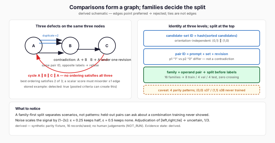
The figure draws duplicates, contradictions and the three-node cycle, and shows why identity needs three levels. Notice that a scalar score cannot satisfy a cycle, and that family separation still leaves parity patterns unseen in training.
Agreement, adjudication and noise
Suppose several judges label the same pair. Let n_left, n_right, n_tie and n_unc be the counts of each answer from N judges. A simple adjudication rule takes the label with the largest count and records agreement as that count divided by N. If two or more labels share the maximum count, the rule returns “uncertain” rather than picking one arbitrarily.
The fixture stores one worked case: three votes, one each for left, right and tie. Every count is 1, three labels share the maximum, and the adjudicated result is uncertain with agreement 1/3. A rule that broke ties by alphabetical order or by the first vote would have returned a strict preference that no majority supported.
Agreement is a description of the judges, not of the truth. Three judges who share a misconception agree perfectly. Low agreement can mean the candidates are genuinely close, the criterion is ambiguous, or the judges are careless. These have different remedies, and none is visible in the agreement figure alone.
A simple model of noisy labelling makes the cost of disagreement explicit. Suppose each strict label is flipped independently with probability ε. A pairwise objective of the kind Chapter 32 derives has, for a pair with model margin m in the true direction, loss −log σ(m) when the label is correct and −log σ(−m) when it is flipped, where σ is the logistic function. The expected derivative with respect to m is
Split by family before any label exists
Supervised chapters split data by family so that variants of one scenario do not appear on both sides of the train/test boundary. Preferences need the same discipline, applied earlier. If candidates are generated and labelled first and the records are split afterwards, it is easy for a family’s comparisons to leak across splits, and for decisions about which comparisons to keep to be influenced by labels the evaluation will later use.
The fixture therefore assigns families to splits before any candidate or label exists. The generator enumerates the sixteen ordered operand pairs (a, b) with a and b in 0 to 3, shuffles them with the seed, and gives the first eight to training, the next four to validation and the last four to the final test. Only then does it build each record’s prompt, candidates and label.
A family-first split protects against one specific failure: the same scenario, reworded or reordered, being learned in training and then credited as generalisation at test. It does not protect against everything that could make the test easy or hard.
- Shared answer strings. Every record has the same two candidates, the
strings
0and1. Sharing them across splits is not leakage; it is the task. But a model that learns “prefer1” learns something that transfers across every family without learning the criterion. - Shared underlying patterns. The criterion depends only on the parities of a and b. Sixteen surface families collapse onto four parity patterns. A family-first split keeps families apart; it does nothing to keep patterns apart, or to ensure that every pattern appears in training.
The second point turned out to matter in the recorded fixture, and Chapter 34 will show why.
| Seed | Split | Parity patterns (a mod 2, b mod 2) present |
|---|---|---|
| 37 | Train | (0,1) ×2, (1,0) ×2, (1,1) ×4 |
| 37 | Validation | (0,0) ×2, (0,1), (1,0) |
| 37 | Test | (0,0) ×2, (0,1), (1,0) |
| 38 | Train | (0,0) ×4, (0,1) ×2, (1,0) ×2 |
| 38 | Validation | (0,1), (1,1) ×3 |
| 38 | Test | (0,1), (1,0) ×2, (1,1) |
At each seed one of the four parity patterns never appears in training but does appear in the held-out splits: (0, 0) at seed 37 and (1, 1) at seed 38. The families are perfectly separated, and yet half of the seed-37 test pairs and a quarter of the seed-38 test pairs ask about a combination the training data never showed. Whether a model can answer them depends on whether it has learned the parity rule or only the three cases it saw. A family-first split is necessary; it is not a guarantee of a representative evaluation.
The recorded fixture
The comparison family is called synthetic-parity-preferences/1. Each record
has a prompt of the form a+b%2?, an educational shorthand that the generator
parses explicitly as “the parity of a plus b”; it is not a claim about any
programming language’s operator precedence. The two candidates are the
strings 0 and 1. Under criterion revision p1 the preferred candidate is
(a + b) mod 2. Revision p2 reverses the criterion. Labels are produced by this
deterministic rule and are marked DETERMINISTIC_SYNTHETIC_CRITERION; the
record of human judgements is explicitly NOT_RUN.
Both seeds produced 16 records: 8 for training, 4 for validation and 4 for the
final test, with no family appearing in more than one split. Training labels
were balanced at both seeds, four preferring 0 and four preferring 1. The
held-out labels were not: at seed 37 the test split had two of each, but at
seed 38 three of the four test pairs preferred 1. That imbalance is a
property of a four-pair test set, and Chapter 32 will show how much it
explains.
Four controlled defects were then introduced into copies of the dataset, and each was refused for its intended reason:
| Control | Construction | Diagnostic |
|---|---|---|
| Duplicate | The first record appended a second time | DUPLICATE_PAIR |
| Contradiction | The first record appended with its label reversed | CONTRADICTION |
| Reversal | The first record’s label reversed in place | LABEL_CRITERION |
| Family overlap | A p2 record for the first record’s operands added to validation | FAMILY_LEAK |
The last control is worth reading closely. The added record has a different pair ID from the original, because its criterion revision differs, so it is neither a duplicate nor a contradiction. It is refused because its family, which is defined by the operands rather than the criterion, already lives in training. Identity at the right level catches it; identity at the pair level would not.
The criterion change is recorded directly. For operands 8 and 9, revision p1
prefers 1 and revision p2 prefers 0, and the two records carry different
pair IDs. If the revision were dropped from the identity, these two records
would look like a contradiction and one of them would be discarded, silently
erasing the policy change.
The fixture also records a synthetic label-noise condition. Two of the eight
training labels, 25%, were flipped, chosen by a seeded random sample. The
flipped rows are marked SIMULATED_ANNOTATOR_NOISE; the clean dataset is not
modified, and no validation or test row is ever corrupted. Tie and uncertain
example records exist as annotation-state controls and are excluded from
strict-pair training, which is the only use the next two chapters make of the
data.
A worked graph
The stored cycle example has three abstract candidates and the edges A → B,
B → C and C → A, where an arrow points from the preferred to the rejected
candidate. A depth-first search that marks nodes “active” while it explores
their descendants finds the cycle when it reaches A again while A is still
active. The fixture records detected: true.
The parity fixture itself cannot contain a cycle under one criterion, because the label for each pair is computed from a fixed rule and each prompt has only two candidates. Cycles appear when more than two candidates exist per prompt, or when records produced under different criteria are pooled. Pooling p1 and p2 records for the same operands without the revision in the identity would produce the two-node version, a contradiction. That is the mechanism to keep in mind for real data: inconsistency often enters at the point where data from different sources, annotators or policy versions is merged.
What the data establishes
The engineering establishes that the comparison layer behaves as specified on the cases it was given: identities are stable and orientation-independent, families are separated before labelling, the four constructed defects are refused for the intended reasons, ties and uncertain records stay out of strict-pair training, and synthetic noise is applied to exactly the declared training rows.
It does not establish that the fixture resembles human preference data. No human judged anything. The tie and uncertainty records illustrate how those states are represented; under the strict parity rule there is no genuine indifference to discover. The adjudication example is a single constructed vote. The noise is synthetic and independent of content, whereas real annotator errors cluster on hard or ambiguous cases.
Limitations
The fixture has sixteen comparisons per seed, built from four parity patterns and two candidate strings. It invites shortcuts by construction, and at each seed one parity pattern is absent from training but present in held-out data. Four test pairs per seed cannot support statistical claims. Agreement, adjudication and cycle detection are demonstrated on constructed examples, not measured on real annotations. A family-first split separates scenarios; it neither balances labels nor guarantees that held-out patterns were seen in training. None of this is evidence about the reliability of any real preference dataset.
FineTuneLab
The comparison layer lives in ftlab.preferences.data in the Part VI
engineering staging package. record builds one sealed comparison with prompt,
candidate, candidate-set and pair identities; generate assigns families to
splits before building records; validate recomputes every record from its
operands and criterion and refuses duplicates, contradictions, criterion
violations, family leakage and unstable candidate identities; adjudicate
implements the counted majority with uncertainty on tied counts; cycles
performs the depth-first cycle check; noise flips a declared fraction of
strict training labels and marks them; and training_rows and
audit_training admit only frozen training records with strict labels. The
experiment that produced the evidence above is dataset_experiment in
ftlab.preferences.experiments, run through examples/part_vi/batch_demo.py
against a frozen plan.
Where this leads
A comparison says that one response is better than another. The next chapter asks how to turn that statement into a gradient for a policy, without first training a separate reward model. The answer, Direct Preference Optimization, is mathematically tidy. The experiment that tests it on this fixture is not, and the reasons it is not trace directly back to what this chapter found in the data: balanced training labels, unbalanced held-out labels, two shared answer strings and four parity patterns.
Further Reading
- Paul Christiano et al., “Deep reinforcement learning from human preferences” (2017). Read the source. Trains agents from human comparisons of behaviour segments with small feedback budgets. Read it as the origin of the comparison signal Part VI inherits.
- Nisan Stiennon et al., “Learning to summarize from human feedback” (2020). Read the source. Fits a reward model to human summary comparisons and optimises the policy with reinforcement learning, beating human references. Read it as the first language-model proof that preferences improve upon demonstrations.
- Yuntao Bai et al., “Training a Helpful and Harmless Assistant with Reinforcement Learning from Human Feedback” (2022). Read the source. Releases the HH preference datasets. Read it as the public data whose pairwise structure the chapter’s identities and split discipline are designed to govern.