Hyperparameters, Overfitting and Forgetting
Treat schedules, effective batch, epochs, regularisation and checkpoint selection as parts of one experiment, read raw validation curves without smoothing, and measure forgetting where it is possible but not forced.
A fine-tuning run reports one final number, and that number depends on a dozen choices: the peak learning rate, how it rises and falls, how many examples contribute to each update, how many times the data is seen, how strongly parameters are pulled towards zero, how much dropout perturbs them, when training stops and which checkpoint is kept. Change any of these and the final number moves. Change several at once and it becomes impossible to say which choice moved it.
This chapter treats those choices as parts of a single experimental contract. It derives what each one does to the update, then runs two controlled experiments. The first deliberately overfits noisy labels and asks what validation-based selection rescues. The second asks whether adapting to a new task damages a previously learned one, in a setting where the damage is possible but not inevitable.
Both experiments contain results that do not support the obvious story. Those results are reported as carefully as the ones that do.
The results below have also been executed in the pinned Docker CPU environment as FT-P5-INTEGRATED-02-28, using the repaired Part IV foundation and local FineTuneLab 0.12.0. The integrated evidence map records source, configuration, environment and artifact hashes for each claim. Earlier staging and authoring comparisons remain historical provenance; they are not independent acceptance. No pretrained-model operation is authorised by these runs.
Index the schedule by optimiser updates
Chapter 10 introduced warm-up and decay and insisted that a schedule be indexed by the optimiser-update counter k, not by microbatches or epochs. The schedule used here is linear warm-up over w updates followed by linear decay to zero at K updates:
Two consequences follow. First, K is part of every rate: stopping a K = 100 schedule at update 60 is not the same as running a K = 60 schedule. Second, a resumed run must restore k exactly or its learning rates shift, a requirement Chapter 30 makes concrete.
Effective batch and epochs are derived quantities
The effective batch is the number of examples whose gradients contribute to one update:
The number of epochs is not an independent setting. It is
The large-minibatch work of Goyal and colleagues proposed scaling the learning rate linearly with batch size and adding a warm-up phase. That is a heuristic established for a particular setting; it is described here but not tested. Changing B_eff without revisiting η is a hyperparameter change, whether or not anyone meant it as one.
Regularisers change the update, not the objective’s meaning
AdamW, from Loshchilov and Hutter and derived in Chapter 10, applies decoupled weight decay: before the adaptive step, each parameter is multiplied by 1 − η_kλ. Over a whole run, an otherwise motionless parameter is shrunk by a factor of
Dropout, from Srivastava and colleagues, multiplies hidden activations during training by a random mask, scaling survivors by 1/(1 − p), and is disabled in evaluation mode. The training metrics in this chapter are measured in evaluation mode, so they describe the deterministic network, not the noisy one the optimiser saw.
Selection must use only the validation split
Early stopping, examined systematically by Prechelt, treats the number of updates as a hyperparameter chosen on held-out data. The rule used here is precise:
- Evaluate training, validation and retention metrics at update 0, every 10 updates and at the end.
- Keep the checkpoint with the lowest validation loss, taking the earliest in a tie.
- Stop after eight consecutive evaluations without improvement.
- Evaluate the test split once, on the selected checkpoint, after selection.
The validator enforces the third and fourth points structurally. A configuration that names any selection split other than validation is refused at construction. The test result is computed only after the selected state is restored, and the validator checks that the reported selection is the true validation minimum of the recorded curve.
Every curve point stores raw logits. The validator recomputes losses, predictions and counts from those logits, checks that evaluation points occur exactly at the declared updates, and rejects a curve whose rows belong to another run. The curves below are those raw points, unsmoothed.
Overfit noisy labels on purpose
The first experiment uses a two-dimensional grid. Training, validation and test splits each contain 16 distinct points; the label is whether the second coordinate is positive. In the training split only, five of the sixteen labels are flipped. A network with one hidden layer of width 16 and tanh activation (65 trainable parameters for this task) is trained under two conditions for up to 160 updates:
- High rate, unregularised: η = 0.12, no weight decay, no dropout.
- Lower rate, regularised: η = 0.02, λ = 0.01, dropout 0.2.
The raw curve for seed 37 under the high rate (training loss, validation loss, training correct of 16, validation correct of 16) is:
| Update | Train loss | Validation loss | Train correct | Validation correct |
|---|---|---|---|---|
| 0 | 0.6976 | 0.7093 | 8 | 7 |
| 10 | 0.5387 | 0.4388 | 12 | 12 |
| 20 | 0.3599 | 0.4222 | 12 | 14 |
| 30 | 0.1805 | 0.5786 | 16 | 12 |
| 40 | 0.0682 | 0.7535 | 16 | 12 |
| 60 | 0.0175 | 0.9779 | 16 | 11 |
| 100 | 0.0078 | 1.1364 | 16 | 11 |
By update 30 the network classifies all sixteen training points “correctly”, including the five whose labels are wrong. It has memorised the noise. Validation loss reaches its minimum at update 20 and then rises for eight consecutive evaluations, so training stops at update 100. The selected checkpoint, from update 20, classified 14 of 16 test points correctly.
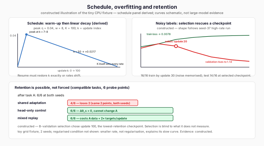
The figure sketches the warm-up and decay schedule, the memorisation gap with its validation minimum at update 20, and the retention branches. It is a constructed illustration of the tiny CPU fixture, not large-model evidence. Notice that validation-based selection rescues a checkpoint after memorisation begins, and that selection remains blind to retention.
Seed 38 behaved the same way: selected at update 20, stopped at 100, 13 of 16 test points correct.
Read the regularised condition honestly
The regularised condition never memorised the noise at seed 37. Training loss fell slowly to 0.4685, validation loss to 0.4164 at update 160, and the best validation loss occurred at the final evaluation. At seed 38 the minimum came at update 140 and validation loss rose slightly afterwards. The selected checkpoints classified 12 of 16 test points correctly at both seeds.
| Seed | Condition | Selected update | Selected validation loss | Test correct |
|---|---|---|---|---|
| 37 | High rate, unregularised | 20 | 0.422157 | 14/16 |
| 37 | Lower rate, regularised | 160 | 0.416379 | 12/16 |
| 38 | High rate, unregularised | 20 | 0.394569 | 13/16 |
| 38 | Lower rate, regularised | 140 | 0.406418 | 12/16 |
The tempting narrative is “regularisation prevents overfitting and so is better”. The evidence does not say that. The unregularised condition overfitted badly after update 20, but early stopping discarded everything after update 20. Its selected checkpoint had a comparable validation loss and a better test count at both seeds.
Nor can the regularised condition’s behaviour be attributed to regularisation. It changes three settings together: a learning rate six times smaller, weight decay whose cumulative effect we calculated at about 1.6%, and dropout. The most plausible single cause of its slow, stable curve is the smaller learning rate, but the experiment cannot separate them. A real ablation would change one setting at a time.
Finally, sixteen test points cannot distinguish 14 from 12 with any confidence. The defensible conclusion is narrow: validation-based selection recovered a reasonable checkpoint from a run that went on to memorise its noisy labels.
Derive why adaptation can interfere
The second experiment concerns forgetting. Consider a network with shared parameters θ_s that compute a representation h(x; θ_s), and two task heads. Suppose task A has been learned and we now take gradient steps on task B’s loss L_B, updating θ_s and B’s head. To first order, the change in A’s loss from one plain gradient step of size η is
Two controls follow directly. If θ_s is frozen and only B’s head trains, then Δθ_s = 0 and A’s predictions cannot change at all, whatever happens to B. If both losses are optimised together (replay), the update follows the gradient of L_A + L_B and is pulled back whenever it would raise A’s loss.
McCloskey and Cohen named the phenomenon catastrophic interference when sequential training of connectionist networks destroyed earlier learning. Kirkpatrick and colleagues later proposed slowing learning on parameters important to earlier tasks. The tension between learning new things and preserving old ones is often called the stability–plasticity dilemma. This chapter measures it rather than cites it.
Make forgetting possible, not forced
Chapter 12’s retention experiment used two rules that contradicted each other on the same inputs: copy versus rotation. A model with no task signal could not satisfy both, so the loss of the first rule was built into the design. That experiment demonstrated the mechanics of adaptation, not a tendency to forget.
The design here removes the contradiction. Task A asks whether the first coordinate is positive; task B asks whether the second is. Both are simultaneously learnable. They have separate heads on a shared tanh layer of width 8. Forgetting is therefore possible, through drift in the shared layer, but not forced: a network exists that solves both.
Retention is measured on six fixed points declared before any training and never used for optimisation or selection. The sequence is:
- Train task A (shared layer and A head, 33 parameters) for 100 updates at peak rate 0.03.
- From that state, run three branches for task B, each selected on B’s
validation loss:
- Shared adaptation: shared layer and B head (33 parameters).
- Head-only control: B head only (9 parameters).
- Mixed replay: shared layer and both heads, optimising A and B losses with equal weight (42 parameters, twice the targets per update).
Read the retention results
Task-A retention counts, each out of the six declared points:
| Seed | Before A training | After A training | After shared B adaptation | B head-only control | Mixed replay |
|---|---|---|---|---|---|
| 37 | 3 | 6 | 4 | 6 | 6 |
| 38 | 1 | 6 | 4 | 6 | 6 |
Before training, the counts are chance-level. Training on A establishes the
capability at both seeds. Shared adaptation to B then loses two of six points at
both seeds, while both controls keep all six. The lost records are the same
two points, retention-1 and retention-2, at both seeds: a shared geometric
failure pattern, not two independent random failures.
The B results show the other side of the trade-off:
| Seed | Branch | Selected B validation loss | B test correct |
|---|---|---|---|
| 37 | Shared adaptation | 0.110637 | 16/16 |
| 37 | Head-only control | 0.574970 | 12/16 |
| 37 | Mixed replay | 0.144204 | 16/16 |
| 38 | Shared adaptation | 0.091832 | 16/16 |
| 38 | Head-only control | 0.476977 | 12/16 |
| 38 | Mixed replay | 0.133153 | 15/16 |
The head-only control is maximally stable and barely plastic: the frozen features were learned for A, so B’s head cannot do much with them. Shared adaptation is maximally plastic and loses some of A. Replay achieves most of both at the cost of A’s data and twice the targets per update.
The raw curve shows when the loss happens. For shared adaptation at seed 37, the retention count stayed at 6 through update 60, fell to 5 at update 70 and to 4 at update 90. At seed 38 it fell to 4 at update 60. Training loss on B was still falling, and B’s validation loss reached its minimum at update 100 at both seeds. The selection rule, which looks only at B’s validation split, chose the checkpoint with the lowest retention. A selection criterion is blind to everything it does not measure.
Data mixing is a hyperparameter
Replay mixed A and B with equal weight by dividing each task’s summed loss by twice the training-set size. Other ratios were not run. The ratio determines both how strongly A is protected and how slowly B is learned, and it changes the number of targets per update. Replay’s success here is therefore a demonstration that a mixed objective can preserve A while learning B, not an estimate of the right mixture.
Distinguish this evidence from Chapter 12’s
The two retention experiments support different kinds of claim.
| Property | Chapter 12 | This chapter |
|---|---|---|
| Tasks | Contradictory on the same inputs | Compatible, different axes |
| Can one network solve both? | No | Yes |
| Forgetting | Forced by design | Possible, observed |
| Controls | Source continuation, later tagged control | Head-only and replay, from the same learned state |
| What it shows | Adaptation mechanics | A shared-representation interference mechanism in one toy setting |
The present evidence is stronger in one respect: the loss is not a logical necessity, and the controls show that it can be avoided by freezing or by replay. It is still a two-seed result on six probe points in an eight-unit network. It does not estimate how much a pretrained language model forgets, and the implementation records a limit stating that it makes no general catastrophic-forgetting claim.
Preserve the negative results
Three findings in this part of the book cut against simple stories, and they remain in the record:
- the regularised condition did not beat the early-stopped unregularised one, and could not have been attributed to regularisation if it had;
- in Chapter 27, the seed-37 retention branch degraded more under continued domain training than under response adaptation, so interference was not isolated there;
- validation-based selection chose the lowest-retention checkpoint in every shared-adaptation run.
A results section that drops these would be shorter and would teach the wrong lessons.
Limitations
The networks are tiny and the data is a finite artificial grid. Each comparison has two seeds. Retention is measured on six points and tests on sixteen. The noisy-label condition flips a fixed set of five labels. No pretrained model is involved. Equal update counts give unequal parameter and target budgets across branches.
The experiment was recorded in the engineering staging environment and re-executed in a separate authoring container against the repaired Part IV package. Every count, selected update, stopping update and learning rate matched exactly. Recorded losses agreed to within about 7 × 10⁻⁷, and raw logits to within about 6 × 10⁻⁵.
FineTuneLab
The experiments live in the module ftlab.advanced.dynamics, integrated
in the local 0.12.0 package. TrainingConfig declares every setting and refuses any
selection split other than validation; rate_at is the schedule;
accumulated_backward implements the summed-loss accumulation; fit trains,
selects and evaluates the test split once; check_measurement and
validate_curve recompute every metric and the schedule from raw evidence. The
recorded curves are also exported as an unsmoothed CSV with seed, condition, run
identity, update and split on every row. These components are included in the locally verified 0.12.0 wheel,
which remains unpublished.
Where this leads
Every run in this chapter fitted on one CPU thread. Effective batch entered only through accumulation. The next chapter, Scaling Beyond One GPU, increases N_d, and with it the memory each device must hold, the communication each update requires and the ways effective batch can change without anyone noticing.
Further Reading
- Ilya Loshchilov and Frank Hutter, “Decoupled Weight Decay Regularization” (2017). Read the source. Decouples weight decay from adaptive updates and improves Adam’s generalisation. Read it for the update whose schedule-dependent shrinkage the chapter quantifies; also recommended in Chapter 10 for the update derivation.
- Lutz Prechelt, “Early Stopping — But When?” (1998). Read the source. Systematises validation-based stopping over more than a thousand runs. Read it as the foundation for the chapter’s earliest-minimum-validation selection rule.
- James Kirkpatrick et al., “Overcoming catastrophic forgetting in neural networks” (2016). Read the source. Protects important weights and learns tasks sequentially. Read it as the principled alternative to the chapter’s replay and head-only controls; also recommended in Chapter 12 for retention measurement.