Exporting, Serving and Measuring the Result
Export the composed model as identity-checked JSON artifacts, reload it, serve it on a bounded loopback HTTP interface whose 24/24 responses match the library, and read each local timing and memory figure against the boundary it actually measures.
Chapter 40 ended with a composed weight in memory, checked against its unmerged form. Nobody can use a tensor that lives in one Python process. To deliver it, the model has to be exported to an artifact, loaded somewhere else, identified as the same model, placed behind an interface with a strict contract, and measured as a running service. Each step can silently change what is being served.
This chapter asks what it takes to turn a model artifact into a reproducible local service. It follows the combined system from Chapter 37 through export, reload and a loopback HTTP server. Every served response is compared with the library’s output for the same request, and the cost of each path is measured. The equivalence result is simple: all 24 HTTP responses matched the library exactly. The measurements need more care. Each timing figure in this chapter measures a different boundary, and comparing two of them without naming the boundaries produces a wrong conclusion.
The integrated record is FT-P7-INTEGRATED-01-41-s37, at data seed 37. It was run on one CPU-only container: Python 3.13.18 and PyTorch 2.6.0 on a 12th Gen Intel Core i9-12900KF under WSL2. The timings are local observations on that machine, not portable benchmarks.
Two kinds of artifact
A LoRA-adapted model can be exported in two forms.
- Adapter-only. The artifact stores the adapter factors, their composition weights and the policy revision. The base model is not included. It must be supplied separately at load time and must be the same base the adapters were built for. Adapter-only artifacts are small and let one base serve many adapters, but they make base identity a load-time dependency.
- Merged. The artifact stores the dense composed weight. It needs no adapter code at load time and cannot be decomposed again, so it no longer records which adapters produced it. Its provenance has to live in its manifest.
The experiment exports both forms of the same combined system and loads both.
Serialisation format is a security decision as well as a convenience. Python’s
pickle, historically PyTorch’s default checkpoint format, can execute arbitrary
code when a file is loaded. Loading an untrusted pickle is therefore equivalent
to running untrusted code (Hugging Face, Pickle Scanning documentation). Formats
such as safetensors store a JSON header and raw tensor buffers and execute nothing
on load. The book’s educational artifacts use the same principle at smaller
scale. The payload is plain JSON. Tensors are encoded as finite numbers with a
declared shape and dtype. Parsing refuses duplicate keys and non-finite constants
such as NaN and Infinity. Nothing in an artifact is ever executed.
The manifest and the identity chain
Each export writes two files: a payload, artifact.json, and a manifest,
manifest.json. The manifest records:
| Field | What it identifies |
|---|---|
| format, kind | the artifact schema and whether it is adapter-only or merged |
| payload, payload_sha256 | the fixed adjacent payload file and the SHA-256 of its bytes |
| contract, policy | the task contract and the policy revision the model serves |
| base_identity | a digest of the frozen base’s state |
| adapter_identity | a digest of the ordered adapter digests |
| model_identity | a digest of base, adapters, weights, policy and merge mode |
| weight_identity | a digest of the composed weight tensor |
| precision | FP64 |
| configuration | revision, composition weights and identities |
| authority | LOCAL_INTEGRITY_ONLY; no authenticated execution |
| digest | a seal over all of the above |
Loading is a sequence of checks, each of which can refuse.
- The manifest’s bytes must hash to a value supplied separately by the caller. A manifest cannot vouch for itself.
- The manifest’s seal must match its contents.
- Format and precision must be supported.
- Contract and policy must match the ones the loader serves.
- The base identity must match a fresh digest of the base actually present.
- The adapter identity must match the identity the caller expects.
- The payload must be the fixed adjacent file, and its bytes must hash to the
manifest’s
payload_sha256. - The payload’s kind and configuration must match the manifest’s.
- The reconstructed model’s identity, and the digest of its composed weight, must match the manifest.
Steps 1, 7 and 9 together form an identity chain. The caller’s pinned hash fixes the manifest. The manifest fixes the payload bytes. The payload, rebuilt, must reproduce the declared model and weight identities. Each hash proves that some bytes are the ones expected. None proves that the expected bytes were approved by anyone. The chain is only as trustworthy as whoever supplied the pinned hash. That is why the manifest’s authority field says what it says, and why Chapter 42 keeps approval in a separate place.
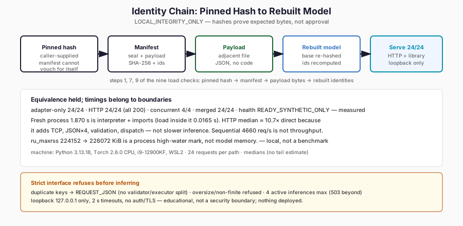
The figure traces the three-link chain (pinned hash to manifest to payload to rebuilt identities) and recalls the serving result: all 24 loopback HTTP responses matched the library. Timings and memory figures in the surrounding table are local single-machine observations, not benchmarks.
A strict interface
The service wraps a loaded model in an inference function with explicit boundaries:
- Parse. Accept at most 32,768 bytes, decode UTF-8, and parse JSON while
refusing duplicate keys and non-finite constants. A failure here gives
REQUEST_JSON. - Validate the request. Require exactly the four declared string fields,
limit the text to 2,048 characters, and require the requested policy revision
to match the active one. A failure gives
REQUEST_SCHEMA,REQUEST_SIZEorPOLICY_REVISION. - Infer. Compute the forward pass without gradient tracking.
- Validate the response. Check the output against the output schema before returning it. A model or wrapper that produced an invalid response would be caught here, not by the client.
Each stage is timed and the timings are returned with the response.
The HTTP layer is Python’s standard-library ThreadingHTTPServer. It handles each
connection in its own thread and binds only to 127.0.0.1, on an ephemeral port.
Nothing is published to another host and the container has no network egress.
It offers two routes: GET /health reports readiness and identities, and
POST /infer runs the inference function. A bounded semaphore admits at most 4
active inferences. A fifth concurrent request is answered at once with HTTP 503
and CONCURRENCY_LIMIT, instead of queueing. Every socket has a 2-second
timeout. Errors from the inference function are returned as HTTP 400 with their
error code, never as a stack trace.
Equivalence: does the service serve the model?
The first question about a service is whether it returns what the library returns. The experiment answered it four ways on the 24 test cases.
| Check | Result |
|---|---|
| Loaded adapter-only service vs in-memory library, outputs | 24/24 equal |
| HTTP responses vs library, outputs and probability vectors | 24/24 equal, all HTTP 200 |
| Concurrent HTTP requests (4 in parallel) | 4/4 HTTP 200, outputs equal |
| Merged export vs library, outputs | all 24 equal |
| Health endpoint | HTTP 200, READY_SYNTHETIC_ONLY, identities match |
The cross-check compared the recorded HTTP bodies with the recorded library outputs field by field, including every probability. It also compared both with an independent reconstruction of the combined system from its factors. Inference is deterministic here: FP64 on CPU, no sampling and no batching effects. Equivalence can therefore be tested as exact equality. With a stochastic decoder or reduced precision, equivalence would have to be defined statistically or with a tolerance, and that definition would itself need to be stated and checked.
Three invalid requests tested the refusal paths:
| Request body | HTTP status | Error |
|---|---|---|
{} |
400 | REQUEST_SCHEMA |
{ |
400 | REQUEST_JSON |
{"operation":"read","operation":"erase"} |
400 | REQUEST_JSON |
The third case matters more than it looks. Many JSON parsers silently keep the
last value of a duplicated key. A request that says read to one component and
erase to another is a classic way to make a validator and an executor disagree.
Refusing duplicates at parse time removes the ambiguity.
Timing: what each number measures
All times were taken with time.perf_counter and are reported in seconds.
| Measurement | Value | What is inside the boundary |
|---|---|---|
| Fresh process, end to end | 1.870156 s | starting a new Python interpreter, importing PyTorch and the library, loading the contract, verifying and loading the adapter-only manifest, printing, exiting |
| Load inside that fresh process | 0.016495 s | manifest and payload verification and reconstruction only |
| Same-process load, adapter-only | 0.015868 s | the same verification and reconstruction in an already-warm process |
| Same-process load, merged | 0.015251 s | as above, for the merged artifact |
| Direct inference, median of 24 | 0.000089926 s | one in-process predict call on the in-memory system: features, forward, softmax, output dictionary; no JSON, no validation |
| HTTP inference, median of 24 | 0.000964179 s | client connection setup, request encoding, loopback TCP, server thread dispatch, parsing, validation, forward, response validation, JSON encoding, response transfer and client decoding |
| Server-side total, median of the 24 HTTP requests | 0.000349 s | parse, validate, forward and validate-response, inside the server thread |
| Concurrent HTTP, 4 requests | 0.0079 to 0.0090 s each | the above, with 4 client threads starting together and contending |
| Sequential service batch, 24 requests | 0.005149 s | 24 in-process service calls including parsing and validation, no HTTP; 4660.68 requests per second |
Several comparisons follow, and each needs its boundary stated.
The fresh-process figure is not “cold-start latency” in the usual sense. It is dominated by starting an interpreter and importing PyTorch. The model load inside that process took 0.016495 s, about 0.88% of the total. It is also not a cold-filesystem-cache measurement. The files had just been written and were almost certainly in the operating system’s page cache. A deployment that keeps a warm process alive would never pay this cost per request. A deployment that starts a process per request would pay it every time.
HTTP is not “ten times slower inference”. The median HTTP figure is about 10.7 times the median direct figure, but the two measure different work. The direct call does no parsing and no validation. The HTTP path adds a TCP connection per request, two JSON encodings, two JSON decodings, schema validation in both directions and thread scheduling. Even the server-side forward stage is not directly comparable with the direct call: it runs on the reloaded model inside a gradient-free context on a server thread, and its median was 0.000183 s. The experiment does not isolate which of those differences accounts for the gap. The model’s arithmetic, a 3 × 4 matrix-vector product, is a negligible fraction of every figure in the table.
The concurrent figures are not throughput. Four requests sent together each took about 8 to 9 milliseconds end to end, roughly 8.5 times a sequential request. That reflects thread start-up and contention in a single process on a tiny workload. It says nothing about how a production server would scale. The 4660.68 requests per second figure comes from 24 sequential in-process calls with no HTTP. It is not a service throughput either.
The distribution matters. The first direct call took 0.000521 s and the fastest 0.0000843 s. With only 24 samples per path, medians are reported because one warm-up outlier would move a mean noticeably. Tail latency, which matters most to users, cannot be estimated from 24 samples.
Portable inference benchmarking requires much more: fixed hardware and software, warm-up protocols, many repetitions, controlled load generators, and percentile reporting under declared load. Industry benchmark suites such as MLPerf Inference define those rules precisely because single-machine timings are hard to compare. Nothing in this chapter meets that standard, and nothing is offered as a benchmark.
Memory: what a high-water mark measures
The experiment read the process’s ru_maxrss before exporting and after
serving. It was 224,152 KiB before and 226,072 KiB after. On Linux, ru_maxrss
is the maximum resident set size the process has ever reached, its
high-water mark. It is not current memory use, and it is not the memory of any
particular object.
The difference of 1,920 KiB is therefore not “the model’s memory”. The model has 12 logical weights in merged form and 26 logical elements unmerged, as counted in Chapter 40. The high-water mark moved because the process imported modules, started threads, ran an HTTP server and allocated buffers, and any of those could have raised the peak. Equally, a model load that happened to reuse freed memory would not move it at all. To measure a model’s memory you need tools that attribute allocations, such as allocator statistics or tensor storage sizes, together with a description of what is shared, duplicated or cached. The readable implementation duplicates the base weight in each LoRA layer: 50 cached parameter elements, where the mathematics needs 26. A storage report must say which of these it counts.
Security limitations, stated plainly
The local server is an educational interface. It has protections, and they have limits.
- Loopback only. The server binds to 127.0.0.1 and refuses any other bind address. Nothing listens on a public interface, and no host port is published.
- Bounded payloads. Requests above 32,768 bytes are refused, and request text is capped at 2,048 characters.
- Socket timeouts. Each connection times out after 2 seconds.
- Bounded active inference. At most 4 inferences run at once.
The semaphore bounds active inferences, not connections or threads.
ThreadingHTTPServer starts a thread for every accepted connection. A client
that opens many connections, or sends headers slowly, can hold threads until
their timeouts expire without ever reaching the semaphore. There is no
authentication, no TLS, no rate limiting and no request logging policy. Python’s
own documentation warns that http.server is not recommended for production,
because it implements only basic security checks. This server is not a security
boundary, and nothing in this chapter should be read as a production deployment.
What the experiment shows and does not show
It shows that the composed model survived export and reload in both forms, with its identity chain verified at every step. It shows that a strict local HTTP interface returned exactly the library’s outputs and probabilities for all 24 cases and for 4 concurrent requests. It shows that malformed and ambiguous requests were refused with explicit codes. And it shows how far apart the cost of the model and the cost of serving it can be on one machine.
It does not show production readiness, scalability, tail latency, security
against hostile clients, portability of the timings, or the memory footprint of
the model. The artifacts are integrity-checked locally. Nobody approved them, and
AUTHENTICATED_EXECUTION = NOT_ESTABLISHED.
Practical lessons
- Export to a format that cannot execute code on load, and seal it with a manifest whose own hash is pinned somewhere else.
- Recompute identities at load time from what was actually loaded, including the base for adapter-only artifacts.
- Validate requests and responses at the service boundary. Refuse duplicate keys and non-finite numbers.
- Test equivalence between the served path and the library on real cases before measuring speed.
- State the boundary of every timing, separate process start from model load, and never compare two figures with different boundaries as if they measured the same work.
- Treat process high-water marks as process facts, not model facts.
Limitations
There was one machine, one container, one data seed and 24 requests per path. The model is a 3 × 4 linear layer, so the serving overhead dominates every measurement. Fresh-process timing includes interpreter start-up and imports and was not taken with a cold filesystem cache. Memory figures are process high-water marks. The HTTP server is the standard-library threading server on loopback, with no authentication or TLS. Nothing was deployed.
FineTuneLab
ftlab.delivery.serving provides export, which writes the payload and the
sealed manifest. It provides load, which runs the identity chain and
reconstructs adapter-only or merged models, and Service, which implements
bounded parsing, validation, inference and timing. It also provides loopback, a
context manager that runs the HTTP server on 127.0.0.1, stops it and verifies
that it stopped. The module can be run as a command to perform the fresh-process
load probe. The experiment is ch41 in ftlab.delivery.experiments.
Where this leads
The service now serves exactly the model it was given, and every artifact can be traced to its identities. None of that says whether the model should be served. Exporting and serving establish that a release is possible. They do not establish that it was reviewed, that anyone authorised it, that it stays healthy once running, or that the previous version can be restored when it is not. Chapter 42, Operating, Auditing and Rolling Back a Fine-Tune, separates those states and tests the last of them.
Further Reading
- Woosuk Kwon et al., “Efficient Memory Management for Large Language Model Serving with PagedAttention” (2023). Read the source. A real serving system showing what proper throughput measurement looks like, and what the chapter’s timings are not.
- Vijay Janapa Reddi et al., “MLPerf Inference Benchmark” (2020). Read the source. The benchmarking rules the chapter explicitly says its single-machine timings do not meet.
- Hugging Face, “Safetensors documentation” (living documentation). Read the source. The safe serialisation format behind the chapter’s no-pickle, nothing-executed-on-load principle; also recommended in Chapter 30 for checkpoint safety.