Statistical Confidence and Ablation
Put a paired, family-clustered bootstrap interval around a difference between systems, show the same 16/24 effect producing a zero-width interval at one data seed and a wide one at another, and keep data-seed, bootstrap-seed and training-seed variation apart.
Chapter 37 ended with a difference that is arithmetically certain. On 24 test cases, the combined system succeeded on all 24 and the base system on 8. The difference is 16/24 and no further computation will change it.
The question this chapter asks is different. How much confidence should we place in an observed difference between two systems? The arithmetic is exact, but the conclusion we want to draw is usually about cases we have not seen. A result can be computed correctly and still support no broad statistical conclusion at all. The gap between those two things is set by the sampling design, the dependence between cases and the number of comparisons made. It also depends on what else changed between the two systems.
The chapter’s most useful result is uncomfortable. The same 16/24 effect, with the same 24 per-case differences, gives a 95% bootstrap interval of zero width at one data seed and an interval running from 10/24 to 20/24 at the other. Nothing about the systems differs between the seeds. Only the grouping of cases into families does.
The integrated records are FT-P7-INTEGRATED-01-38-s37 and FT-P7-INTEGRATED-01-38-s38. They compare the sealed evaluations from Chapter 37’s records at the same data seed, and the comparisons were checked to bind to those evaluation digests. As before, the adapters are constructed, not trained.
Paired differences
Two systems are evaluated on the same n cases. For case i, let sᵢ(L) and sᵢ(R) be 1 if the left or right system succeeds and 0 if not. The paired difference is
Pairing matters for the variance, not the point estimate. The unpaired and paired estimators give the same Δ̂, but
The bootstrap
The bootstrap (Efron, 1979) estimates the sampling variability of a statistic by treating the observed sample as a stand-in for the population. It draws B new samples of the same size, with replacement, from the observed one. It recomputes the statistic on each, and studies the spread of the B values. A percentile interval at level 1 − α takes the α/2 and 1 − α/2 quantiles of that spread.
The implementation uses B = 400 replications and α = 0.05. Quantiles use linear interpolation between order statistics. For sorted values v₀ ≤ … ≤ v_{B−1}, the q-quantile is
Paired bootstrap resampling is standard practice for comparing systems on a shared test set. Koehn (2004) is an early and widely used statement of it for machine translation. The resampled object is the pair, never the two systems separately, so each replicate preserves the covariance.
Two cautions belong here, before any numbers. First, a percentile interval is a procedure. If the sampling assumptions held, intervals constructed this way would contain the true difference in roughly 95% of repeated experiments. A single realised interval does not contain the true value “with 95% probability”. The value is fixed, and the interval either contains it or does not. Second, the repeated-sampling guarantee is asymptotic and weak in small samples. With 8 independent units, the experiment below cannot validate the nominal coverage, and it does not try to.
The statistical unit
The bootstrap’s central assumption is that the resampled units are independent draws. The 24 test cases are not independent. They come in families of three consecutive cases. In a real dataset, a family might be several items written by the same annotator, several paraphrases of one source document, or several turns of one conversation. Cases within a family share causes of success and failure.
When observations are clustered, the variance of a mean depends on the correlation inside clusters. For m observations per cluster, with common variance σ² and intra-cluster correlation ρ, the variance of the overall mean of n observations is
The implementation therefore resamples families, not cases. With 8 families,
each bootstrap replicate draws 8 families with replacement, pools their per-case
differences, and takes the example-weighted mean. Because every family here has
three cases, that equals the mean of the 8 family means. The random generator is
Python’s random.Random, seeded explicitly, and families are drawn from a sorted
key list so that the draw sequence is reproducible. A request for case-level
resampling is refused (CLUSTER_REQUIRED) whenever any family contains more than
one case.
What the comparisons produced
Four comparisons were declared before the run. Each was evaluated at two data seeds and two bootstrap seeds, with 400 replications each time.
- Positive: base → combined.
- Small: single fault → combined. The two differ in one delivered output.
- Null: combined → combined.
- A ablation: base → adapter A.
| Comparison | Effect | Data seed | Bootstrap seed 37 | Bootstrap seed 38 |
|---|---|---|---|---|
| Positive | 16/24 | 37 | [16/24, 16/24] | [16/24, 16/24] |
| Positive | 16/24 | 38 | [10/24, 20/24] | [10/24, 22/24] |
| Small | 1/24 | 37 | [0, 0.125] | [0, 0.125] |
| Small | 1/24 | 38 | [0, 0.125] | [0, 0.125] |
| Null | 0 | 37 | [0, 0] | [0, 0] |
| Null | 0 | 38 | [0, 0] | [0, 0] |
| A ablation | 4/24 | 37 | [1/24, 6/24] | [1/24, 7/24] |
| A ablation | 4/24 | 38 | [1/24, 6/24] | [1/24, 7/24] |
The intervals are shown as exact fractions of 24 where they are exact. In decimals, 16/24 is 0.667, 10/24 is 0.417, 20/24 is 0.833 and 22/24 is 0.917. The authoring cross-check reimplemented the resampling, quantiles and pairing without importing the library. It reproduced all 400 draws of every comparison exactly, as well as each effect and interval endpoint.
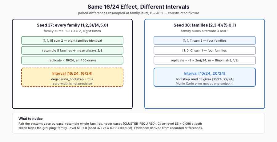
The figure shows why the grouping decides the interval. It is derived from the recorded paired differences: every seed-37 family sums to 2, so resampling cannot vary, while seed-38 families alternate between 3 and 1, so the same 16/24 effect yields [10/24, 20/24]. The zero-width case is flagged degenerate, not precise.
A zero-width interval
At data seed 37 the positive comparison is degenerate: every one of the 400 replicates equals 16/24. The reason is visible in the family sums of the differences. The seed-37 test partition starts at pattern 1, so its families contain patterns (1, 2, 3) and (4, 5, 0) in alternation. The base system fails patterns 2 to 5 and the combined system fails none, so every family contains exactly two differences of 1 and one of 0. Every family mean is 2/3. Any resample of 8 families therefore has mean 2/3.
At data seed 38 the partition starts at pattern 2, and the families are (2, 3, 4) and (5, 0, 1). The first kind has three differences of 1, the second only one. The per-case differences are the same multiset as before, 16 ones and 8 zeros, but the family sums now alternate between 3 and 1. If m of the 8 resampled families are of the first kind, the replicate mean is
The analytical standard errors make the contrast explicit. They are derived from the recorded differences, not from any additional run. If the 24 cases were resampled independently, the standard error of the mean of 16 ones and 8 zeros would be √((2/3)(1/3)/24) ≈ 0.096 at both seeds. Family resampling gives 0 at seed 37. At seed 38, where the family means are 1 and 1/3, it gives (1/3)/√8 ≈ 0.118. The seed-37 arrangement behaves like negative intra-family correlation, because each family balances successes against failures. The seed-38 arrangement behaves like positive correlation. The same 24 numbers carry different information depending on how they are grouped.
So a zero-width interval does not mean zero uncertainty. It means that the
resampling procedure, applied to this sample, produced no variation. Real
uncertainty, about other families, other patterns or other tasks, is not
represented in the procedure at all. With 8 constructed families whose structure
is periodic, the procedure has very little to work with. The implementation
flags every such case as degenerate_bootstrap = true, so the zero width cannot
be mistaken for precision.
The small control
The single fault differs from the combined system in one delivered output, so one family has a difference sum of 1 and the other seven have 0. A replicate mean is k/24, where k counts how often that family is drawn, with k ~ Binomial(8, 1/8). Because P(k = 0) = (7/8)⁸ ≈ 0.344, which is well above 0.025, the lower endpoint is 0. Because P(k ≥ 3) ≈ 0.067 but P(k ≥ 4) ≈ 0.011, the upper endpoint is 3/24 = 0.125. The interval [0, 0.125] was reproduced at both data seeds and both bootstrap seeds.
The interval includes zero, and the effect, 1/24 ≈ 0.042, is below the practical threshold of 0.1 declared in the configuration before the run. Neither fact says the fault does not matter. At seed 38 the fault executes a disallowed erase. Statistical size and practical consequence are different axes. A single unsafe action can matter more than a large average gain.
The ablation
Adapter A alone against the base differs on the 4 certain-erase cases. Those fall one to a family in alternate families at both seeds, so the family sums alternate between 1 and 0. The replicate mean is m/24 with m ~ Binomial(8, 1/2), and the interval is [1/24, 6/24] at bootstrap seed 37 and [1/24, 7/24] at bootstrap seed 38. The effect, 4/24 ≈ 0.167, exceeds the practical threshold.
Three kinds of seed
This experiment involves three different random seeds. Only two of them did anything.
- Data seed (37 or 38). It decides how the fixture’s patterns are arranged into families. Changing it changed the positive interval from zero width to [10/24, 20/24]. Data-seed variation is variation in which sample was drawn.
- Bootstrap seed (37 or 38). It decides which families the resampler picks. Changing it moved one endpoint from 20/24 to 22/24 and another from 6/24 to 7/24. Bootstrap-seed variation is Monte Carlo error in computing the interval. More replications shrink it, and it says nothing about the systems.
- Training seed. It does not exist here. Nothing was trained, so there is no variation from initialisation, data order or optimisation noise. In a real fine-tuning comparison, training-seed variance is often the largest source of disagreement between runs, and a bootstrap over test cases does not capture it at all. Estimating it requires training several times.
A report that says “the result was stable across seeds” without saying which seed was varied has said very little. The limitations recorded with the experiment make the same point: the constructed models have no training-seed variability, and bootstrap variability is a different quantity.
Many comparisons
Every additional comparison is another chance for a spurious difference. If k independent tests are each run at level α, the chance of at least one false rejection when all nulls are true is 1 − (1 − α)ᵏ. The Holm procedure (Holm, 1979) controls that family-wise error rate in the strong sense, with more power than plain Bonferroni. Sort the k p-values in increasing order, p₍₁₎ ≤ … ≤ p₍ₖ₎, and set
The implementation checks the arithmetic on a declared fixture of three
p-values, (0.01, 0.04, 0.03). Sorted, they are 0.01, 0.03 and 0.04. The
multiplied values are 3 × 0.01 = 0.03, 2 × 0.03 = 0.06 and 1 × 0.04 = 0.04. The
running maximum gives 0.03, 0.06 and 0.06. In the original order, the adjusted
values are (0.03, 0.06, 0.06), which matches R’s p.adjust with
method = "holm". The record labels these values
MATHEMATICAL_FIXTURE_NOT_EXPERIMENTAL_PVALUES. The experiment computed no
p-value for any system comparison, and none should be inferred.
Ablation and confounding
An ablation removes or changes one component and measures the consequence. It supports a causal reading only if exactly one thing changed. Compare two configurations:
| Configuration | Weight on A | Weight on B |
|---|---|---|
| Combined | 1.0 | 1.0 |
| B removed | 1.0 | 0.0 |
| Weak B | 1.0 | 0.3 |
Combined against “B removed” changes one declared variable, the B weight. The
implementation records it as ONE_VARIABLE_ABLATION, and the difference in task
success can be attributed to B, given everything else that was held fixed.
Suppose instead that a comparison changes the B weight and the policy
revision, or the B weight and the dataset. Then the implementation raises
ABLATION_CONFOUNDED and refuses to label the comparison an ablation. The
record keeps that diagnostic as a negative control.
Confounding also enters through the evaluation. If the left and right evaluations use different test cases, a difference in scores mixes the effect of the system with the effect of the data. That is why pairing is enforced, and why an “unpaired” comparison of two separately reported accuracies is not an ablation even when only one model component changed.
Interpreting the intervals
What may be said about the positive comparison? The combined system succeeded on 16 more of these 24 cases than the base. Under family resampling of this fixture, the interval was degenerate at one data seed and [10/24, 20/24] or [10/24, 22/24] at the other, depending on the bootstrap seed. The procedure has 8 units, a periodic structure and no training variability. Its nominal 95% coverage has not been validated.
What may not be said: that the combined system is significantly better in any population sense; that the true improvement lies in [10/24, 20/24] with 95% probability; or that adapter composition improves fine-tuned models. The experiment can support none of these. The perfect rule baseline from Chapter 37 also scored 24/24, and a comparison against it would show no improvement at all.
Practical lessons
- Fix the statistical unit before computing anything, and resample at the level where independence is plausible. That level is usually the source document, conversation, user or template, not the individual example.
- Pair comparisons on identical cases, and make the pairing checkable through dataset and label identities.
- Flag degenerate intervals instead of reporting them as precision.
- Report which seed varied. Use enough bootstrap replications that Monte Carlo error is small compared with the interval, and use multiple training runs to estimate training variability.
- Declare the comparisons and the practical threshold before the run, and adjust for multiplicity when more than one comparison supports a claim.
- Treat an ablation as causal only when exactly one variable changed.
Limitations
The test set has 8 families of 3 constructed cases per data seed. The adapters
are constructed, so there is no training-seed variation and no learning to
estimate. The percentile bootstrap with 8 clusters has unknown and probably poor
coverage, and the experiment does not establish population coverage. The Holm
values are an arithmetic fixture, not experimental p-values. The practical
threshold of 0.1 is a declared configuration value, not a derived quantity. The
records carry AUTHENTICATED_EXECUTION = NOT_ESTABLISHED.
FineTuneLab
ftlab.delivery.statistics provides compare, which checks sealing and pairing
and runs the family-cluster percentile bootstrap. It also returns the per-case
differences, all draws, the effect, the interval and a degeneracy flag. The
module also provides holm and ablation. The experiment is ch38 in
ftlab.delivery.experiments. It consumes the Chapter 37 evaluations for the same
data seed.
Where this leads
Every interval in this chapter describes variation within one fixed distribution: the same six patterns, the same policy and the same request format. A well-measured in-distribution result can still fail as soon as the inputs, the policy or the surrounding system change. Chapter 39, Generalisation, Shift and Adversarial Tests, challenges the same systems with transformed inputs, an unknown operation, ambiguous requests, injected instructions and a policy revision.
Further Reading
- Bradley Efron, “Bootstrap Methods: Another Look at the Jackknife” (1979). Read the source. The original bootstrap paper, clarifying what a resampling interval is as a procedure with repeated-sampling behaviour.
- Christopher A. Field and Alan H. Welsh, “Bootstrapping Clustered Data” (2007). Read the source. The theory behind resampling families rather than cases, explaining the chapter’s zero-width versus wide interval contrast.
- Rotem Dror et al., “The Hitchhiker’s Guide to Testing Statistical Significance in Natural Language Processing” (2018). Read the source. A practical protocol for choosing paired tests and handling multiple comparisons in NLP settings.