Direct Preference Optimization From First Principles
Derive the DPO loss from the Bradley–Terry model and the KL-regularised reward objective, explain every term and its gradient, and run it on a tiny random policy where the training objective falls but held-out preference agreement does not move.
Chapter 31 ended with a set of strict comparisons: for each prompt x, a preferred response y_w and a rejected response y_l. The classical way to train on them, which Chapter 34 builds in full, has two stages. First fit a reward model that scores responses so that preferred ones score higher. Then use reinforcement learning to move a policy towards responses the reward model likes, while a penalty keeps the policy close to where it started.
Direct Preference Optimization, introduced by Rafailov and colleagues in Direct Preference Optimization: Your Language Model is Secretly a Reward Model, removes both the separate reward model and the reinforcement-learning loop. It shows that, under the same assumptions the two-stage method makes, the optimal policy can be written in closed form, and the reward can be rewritten in terms of that policy. The preference data can then train the policy directly with a loss that looks like binary classification.
This chapter derives that loss term by term, works its gradient by hand, and then runs it. The run is deliberately small enough to inspect completely, and its result is not the usual success story: the training objective decreases at both seeds, and held-out preference agreement does not change at all. Why it does not change is the most useful thing the chapter has to teach.
The measured results were recorded as FT-P6-INTEGRATED-02-32-s37 and FT-P6-INTEGRATED-02-32-s38, in the pinned CPU container, on a randomly initialised policy. The integrated runs are bitwise-identical to the preserved historical records FT-P6-CODEX-03-32-s37/s38; they are not results about any pretrained or aligned language model.
Policies, references and sequence probabilities
A policy π_θ is the model being trained: given a prompt x it assigns a probability π_θ(y | x) to every complete response y. For an autoregressive model, that probability is the product of the next-token probabilities along the response, so its logarithm is a sum:
A reference policy π_ref is a frozen copy of a policy, normally the supervised fine-tuned model that preference training starts from. It receives no gradient, and its parameters must not share storage with the policy being trained; otherwise an update to one silently changes the other.
The assumption behind the method
DPO starts from the same two modelling assumptions as classical RLHF.
The first is a model of how preferences arise. The Bradley–Terry model, from Bradley and Terry’s 1952 paper Rank Analysis of Incomplete Block Designs: I. The Method of Paired Comparisons, assumes each response has a scalar reward r(x, y) and that the probability of preferring y_w to y_l depends only on the difference:
The second is the objective the policy should optimise: high reward, but without drifting far from the reference.
Derive the optimal policy
Fix one prompt x and drop it from the notation. The objective for that prompt is
The key step is to read this equation the other way round. Take logarithms and rearrange:
The loss
Substitute the policy expression for the reward into the Bradley–Terry probability, replace the unknown optimal policy by the trainable π_θ, and maximise the log-likelihood of the observed preferences. Writing c = log π_θ(y_w | x), r = log π_θ(y_l | x), and c₀ and r₀ for the same quantities under the frozen reference, the per-pair margin is
- c − r is the policy’s preference between the two responses, in log probability. It is positive when the policy already prefers y_w.
- c₀ − r₀ is the reference’s preference between the same two responses. It is a fixed number for each pair.
- Their difference is how much the policy’s preference has moved relative to where the reference started. The quantity β log(π_θ/π_ref) for one response is the implicit reward the method fits.
- β scales the margin, which sets both how hard the loss pushes and how far the policy can move before the push fades.
- −log σ is the negative log-likelihood of the observed preference under the Bradley–Terry model.
This is the objective implemented in the book: completion log probabilities are summed over target positions including EOS, the reference values are computed with gradients disabled, and the loss is averaged over pairs.
A worked example
Take β = 0.2, policy log probabilities c = −1 and r = −2, and a reference that assigns both responses −2. The policy’s preference is c − r = 1, the reference’s is 0, so m = 0.2 × (1 − 0) = 0.2 and
When the policy and reference are identical, every margin is exactly zero and every pair’s loss is log 2. This is not a statement that the two responses have equal probability. It only says the policy has not yet moved.
The gradient
Since d/dm[−log σ(m)] = −σ(−m), the chain rule gives
The weight σ(−m) is the model’s current probability of getting the pair wrong under its own implicit reward. It is close to 1 for pairs the policy misorders and decays quickly once the pair is ordered correctly:
| Margin m | Weight σ(−m) |
|---|---|
| −2 | 0.880797 |
| 0 | 0.500000 |
| 2 | 0.119203 |
| 5 | 0.006693 |
| 10 | 0.000045 |
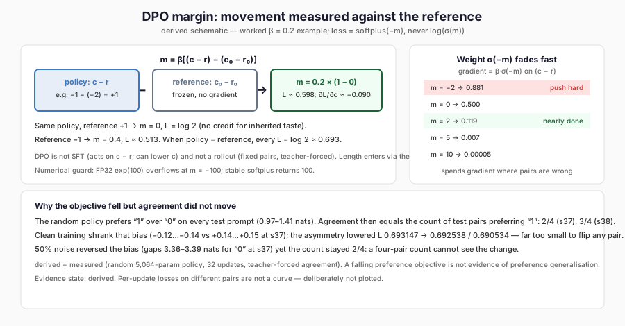
The figure composes the margin from policy and reference preferences and shows how the gradient weight fades. Notice that an inherited preference earns no loss reduction, and that the small bias shift here could not flip any held-out pair.
This is the answer to “what happens when the preferred response already has a much greater relative likelihood?” The pair contributes almost nothing. DPO spends its gradient on pairs it currently gets wrong or nearly wrong, which is the behaviour of logistic regression, not of supervised maximum likelihood.
Three consequences follow from the form of the gradient.
DPO is not SFT with a different label. Supervised fine-tuning on y_w raises c without regard to anything else. DPO acts only on the difference c − r. It can lower c, if r falls faster, and still reduce its loss. The absolute probability of the preferred response is not what the objective protects.
DPO is not a reinforcement-learning rollout. The derivation starts from a reinforcement-learning objective, but training never samples a response from π_θ. It scores two fixed responses per prompt under teacher forcing and takes a gradient step on a classification-style loss. Whatever the policy would generate on its own does not enter the loss.
Sequence length enters through the sum. A longer response accumulates more negative log-probability terms. Two responses of different lengths can have very different c and r for reasons unrelated to quality. The reference term partly cancels this, because the reference sees the same lengths, but only partly. Chapter 33 examines methods that normalise by length instead. In the experiment below every candidate has exactly two target tokens, one content byte and EOS, so length plays no role in these results.
Numerical stability
The loss should be computed as softplus(−m) = log(1 + exp(−m)), never as log(σ(m)) with σ evaluated first. For a confidently wrong pair, say m = −100, the naive form computes 1/(1 + exp(100)). In FP32, exp(100) overflows to infinity, σ evaluates to zero, log(σ) becomes −∞ and the loss is infinite. A stable softplus returns 100. Sequence log probabilities should likewise be accumulated from per-token log-softmax values rather than by multiplying probabilities.
The reference log probabilities are inputs, not parameters. They are computed
under torch.no_grad, and the implementation refuses a reference tensor that
requires gradients and refuses a reference model that shares any parameter
storage with the policy or whose state digest changed during training.
The experiment
The policy is the book’s TinyTransformer at width 8, one block and two attention heads: 5,064 parameters, all trainable, randomly initialised. It is not a supervised fine-tuned model, and it has never seen text. The reference is a frozen deep copy, 20,256 bytes of FP32 parameters with no gradients, verified unchanged before and after training.
The data is Chapter 31’s comparison fixture. Each of the 32 updates uses one training pair, cycling through the eight training pairs four times. Settings are fixed in advance: β = 0.2, AdamW at learning rate 0.01 with no weight decay, gradient-norm clipping at 10 and FP32 arithmetic. No configuration was chosen by looking at validation or test results, and training always stops at the fixed final update.
A second, noisy condition repeats the run after flipping 50% of the training labels, four of eight, chosen by a seeded sample. Chapter 31 showed that at 50% flipping the expected signal is zero.
The outcome measure is held-out preference agreement: on each held-out pair, score both candidates teacher-forced under the trained policy and count the pair as agreeing if log π_θ(y_w) > log π_θ(y_l). This compares the policy’s own log probabilities, not the reference-adjusted margin. It measures which of two fixed strings the policy prefers, not what it would generate.
| Seed | Condition | Test before | Test after | Validation before | Validation after |
|---|---|---|---|---|---|
| 37 | Clean | 2/4 | 2/4 | 2/4 | 2/4 |
| 37 | Noisy | 2/4 | 2/4 | 2/4 | 2/4 |
| 38 | Clean | 3/4 | 3/4 | 1/4 | 1/4 |
| 38 | Noisy | 3/4 | 3/4 | 1/4 | 1/4 |
Training-pair agreement was 4/8 before and after in all four runs.
The training objective tells a different story. Recomputed from the stored per-pair log probabilities over all eight training pairs, with the starting policy as reference, the clean objective was exactly log 2 ≈ 0.693147 before training at both seeds, as it must be when policy and reference coincide. After 32 updates it was 0.692538 at seed 37 and 0.690534 at seed 38. It decreased, slightly, and held-out agreement did not move.
The per-update losses recorded during training cannot substitute for this calculation. Each update sees a different pair, so the first and last recorded losses concern different comparisons, and treating them as a curve would compare unlike quantities.
Why nothing moved
The stored log probabilities show what the policy actually learned. Before
training, at seed 37, the policy assigned the string 1 a higher log
probability than 0 on every test prompt, by between 0.972 and 0.976 nats.
After training the gap had shrunk to between 0.817 and 0.849 nats, still
favouring 1 everywhere. At seed 38 the gap was between 1.33 and 1.39 nats
before and between 1.28 and 1.41 nats after, again favouring 1 on every
test prompt.
The random policy has a preference, but it is almost entirely
prompt-blind: it prefers one answer string regardless of the question.
For such a policy, held-out agreement is fixed by the test labels, not by
learning. It equals the number of test pairs whose preferred candidate is 1.
Chapter 31 found two such pairs at seed 37 and three at seed 38. Those are
exactly the counts in the table, before and after.
The clean training labels are balanced, four preferring each string, so a
global preference for either string earns no reduction in the training
objective. The only way to lower the loss substantially is to learn a
prompt-dependent rule. In 32 small updates the policy mostly shrank its string
bias instead. At seed 37 the four training pairs that prefer 0 each gained
between 0.14 and 0.15 nats of policy margin relative to the reference, and the
four that prefer 1 each lost between 0.12 and 0.14. Because the logistic loss
is convex, a symmetric shift of that kind would raise the average loss; the
small asymmetry between the gains and the losses is what lowered it by a few
ten-thousandths. Nothing approached the size needed to reverse a held-out
pair.
The noisy condition confirms the mechanism from the other side. At seed 37 the
seeded corruption left six of the eight training pairs preferring 0. The
policy duly learned a strong prompt-blind preference for 0: on every test
prompt the gap swung to between 3.36 and 3.39 nats in favour of 0. Measured against the
corrupted labels it was trained on, its objective fell from 0.693147 to
0.567108. Measured against the clean labels it rose to 0.785599. On the test
set, every pair’s ordering reversed, and the count stayed at 2/4, because the
test set happens to contain two pairs of each kind. At seed 38 the corruption
left the training labels balanced, four and four. The policy’s preference for
1 shrank, to between 0.96 and 1.25 nats on the test prompts, without
reversing, and its objective was 0.684314 against the corrupted labels and
0.693856 against the clean ones.
So the noisy condition did not leave the policy untouched. It changed the policy’s preferences more than clean training did, in the wrong direction, and the held-out count was blind to it. A four-pair agreement count could not distinguish a policy that had learned nothing, a policy whose bias had reversed, and, in principle, a policy that had learned the rule for two pairs and broken two others.
What the experiment establishes
The run establishes that the implementation behaves as the derivation says. The objective starts at log 2 when policy and reference coincide; the reference stays frozen and separate; gradients flow only into the policy; the largest gradient norm, 0.485 at seed 37 and 0.803 at seed 38 in the clean runs, stayed well below the clipping threshold; and the trained policy moved in the direction the training labels pushed it.
It establishes that a decreasing preference objective is not evidence of preference generalisation. Here the objective fell while held-out agreement did not move, and in the noisy condition the policy changed substantially while held-out agreement did not move either.
It does not establish that DPO fails. Several features of the setup could each contribute, and the experiment isolates none of them: a randomly initialised policy with no language knowledge rather than a supervised starting point, eight training pairs, 32 updates at a small β, two answer strings that make a prompt-blind bias the easiest thing to learn, and a test set too small to register anything but large changes. Changing any one of these could change the result. A claim about which one matters would need an experiment that changes it alone.
Limitations
The policy is a 5,064-parameter random byte Transformer, not a fine-tuned language model. Candidates are scored teacher-forced; nothing is generated. All candidates have the same length, so the length effects discussed above are derived, not observed. Held-out agreement uses four test pairs per seed, and its value here is determined by the test labels’ composition. The noisy condition flips exactly four training labels, whose effect depends on which four. No separate SFT stage, β sweep, learning-rate sweep or larger dataset was run, and no trainer library was used or compared against.
FineTuneLab
The objective is dpo in ftlab.preferences.objectives. It validates that
all four inputs are equal-length, finite, non-positive log-probability vectors
and that the reference inputs carry no gradient, then returns softplus(−m)
averaged over pairs together with the per-pair margins. sequence_logps
computes summed or mean completion log probabilities from logits through the
existing causal_terms, refusing a mask that does not end in EOS or that
differs from the recompiled completion-only mask. reference_guard refuses a
reference that aliases the policy, holds gradients, shares storage or has
changed state. offline_preference in ftlab.preferences.experiments runs
the fixed-budget experiment, measures every split before and after, and
records the starting, reference and final policy digests, trainable-parameter
audit and per-update history.
Where this leads
DPO is one answer to “how should a comparison become a gradient?” It sums log probabilities, needs a reference, and uses one particular link between reward and probability. Each of those choices can be made differently. The next chapter runs three objectives that make different choices, on the same starting policy and data, and finds that one of them makes held-out agreement worse while its own training objective improves.
Further Reading
- Rafael Rafailov et al., “Direct Preference Optimization: Your Language Model is Secretly a Reward Model” (2023). Read the source. Derives the closed-form policy update that removes the reward model and RL loop. Read it for the inversion the chapter reconstructs term by term; also cited in Chapter 1 as the preference-learning distinction.
- Ralph A. Bradley and Milton E. Terry, “Rank Analysis of Incomplete Block Designs: I. The Method of Paired Comparisons” (1952). Read the source. Models paired comparisons as a logistic function of score differences. Read it for the transitivity assumption that cyclic data violates.
- Hugging Face contributors, “DPO Trainer (TRL documentation)” (living documentation). Read the source. Provides the reference DPOTrainer implementation. Read it to see how production code handles the masking and reference-probability details the chapter builds from scratch.