Evaluation That Measures the Task
Separate the model's probabilities from the system's delivered result, derive every task metric with its own denominator, and show a controlled postprocessor fault that lowers task success to 23/24 while the model's negative log-likelihood stays at 0.284779.
Part VI ended with a policy that earned its whole reward while serving none of the requests it should have served. Its training loss fell and the number being optimised rose. Nothing in either number said that the task had failed. Only an evaluation built around the task, with every outcome counted against its own denominator, revealed what had happened.
Part VII makes that evaluation the subject. Its central question is how we know whether an adapted system is genuinely better, how we deliver it, and how we recover when something goes wrong. The six chapters follow one small workflow through six stages: measure, compare, challenge, compose, serve and operate. This first chapter asks the most basic question of the six. What does it mean for a model, or a system built around a model, to perform the intended task correctly?
The answer has more parts than a single accuracy figure. A model assigns probabilities. A decision rule turns probabilities into an action. A wrapper turns the action into a structured response with a citation. A contract says which responses count as correct. Each of these is a different boundary, and a measurement taken at one boundary cannot see an error introduced at another. The chapter’s central worked example makes that concrete. A deliberately faulty postprocessor corrupts one response out of 24. Delivered task success falls from 24/24 to 23/24. The model’s negative log-likelihood does not move at all: it is 0.284779 before the fault and 0.284779 after it.
The integrated records are FT-P7-INTEGRATED-01-37-s37 and FT-P7-INTEGRATED-01-37-s38, one for each data seed. They were regenerated from the integrated candidate in offline Docker CPU. The original engineering records remain preserved as FT-P7-CODEX-02. Nothing in this chapter involves training. Every adapter is constructed by writing down its weights, so the experiment measures evaluation machinery, not the outcome of fine-tuning.
A task written down
Evaluation starts with a task definition precise enough to be wrong about. The
running example is a benign synthetic docket workflow. Each request names an
operation (read, copy, erase or something else), a certainty
(certain or not), the policy_version the requester believes is in force, and
some free text. A trusted policy, held separately and identified by a SHA-256
digest, decides what should happen.
Under policy revision p1:
- a certain
readorcopyshould be completed; - a certain
eraseshould be refused; - anything uncertain, and any unknown operation, should go to review.
The response is a small structured object with three fields: an action from
{complete, refuse, review}, a boolean abstain that must be true exactly when
the action is review, and a citation that must equal the digest of the policy
actually in force. The output schema forbids extra fields.
The fixture is generated per data seed. Each seed produces 12 training cases, 12 validation cases and 24 test cases. Cases are built from six request patterns in rotation, and every three consecutive cases form a family. The 24 test cases therefore fall into 8 families, and no family crosses a partition. The labels are derived from the request and the trusted policy, and they are stored separately from the inputs, behind a label authority that the system being evaluated never sees.
| Pattern | Operation | Certainty | p1 requires | Test cases per seed |
|---|---|---|---|---|
| 0 | read | certain | complete | 4 |
| 1 | copy | certain | complete | 4 |
| 2 | erase | certain | refuse | 4 |
| 3 | read | uncertain | review | 4 |
| 4 | erase | uncertain | review | 4 |
| 5 | unknown | certain | review | 4 |
The data seed only shifts where the rotation starts. Seed 37 begins the test partition at pattern 1 and seed 38 at pattern 2. The 24 test cases contain the same multiset of patterns at both seeds, arranged into different families. That detail will matter in Chapter 38.
This fixture is deliberately finite. Its six patterns repeat, the partitions exist to demonstrate isolation and data-access discipline, and nothing about it can establish semantic generalisation.
Six systems and an oracle
Every model in the experiment shares one tiny architecture. A request becomes a four-dimensional feature vector
Two rank-1 LoRA adapters are constructed on top of it. Each adds ΔW = (α/r)·B·A with α = r = 1:
- Adapter A has A = [0, 0, 1, 0] and B = [−2, 2, 0]ᵀ. It looks only at the
erase feature, lowering the
completescore by 2 and raisingrefuseby 2. - Adapter B has A = [0, 0, 0, 1] and B = [−3, 0, 3]ᵀ. It looks only at the
uncertainty feature, moving 3 units of score from
completetoreview.
The combined system applies both adapters with weight 1. A weak-B control applies A with weight 1 and B with weight 0.3. Nobody fitted these numbers to data. They were chosen so that each adapter carries one identifiable behaviour, and the evaluation can then be checked by hand.
Two further systems complete the comparison.
- The rule baseline applies the trusted policy directly. It shares the oracle that produced the labels, so it is perfect by construction. It emits a one-hot probability vector and always cites the right policy. Its 24/24 is not an achievement. It is a check that the evaluation can award full marks, and a reminder that a finite rule-defined task can be solved without any model at all. It remains an explicit no-training comparator throughout Part VII.
- The single-fault system is the combined model followed by a postprocessor
with a deliberate bug. For the one test request whose text ends in
test-0, it flips the emitted action (a non-refusal becomesrefuse, a refusal becomescomplete), setsabstainto false, and leaves the model’s probabilities untouched.
Every number in the next sections can be predicted from the weights before running anything, which is the reason for building the systems this way. Take pattern 2, a certain erase, with x = [0, 0, 1, 0]. The base scores are (1, 0, 0), so the base completes it, which is wrong. Adapter A changes the scores to (−1, 2, 0) and refuses it, which is right. Adapter B does not touch the erase feature, so B alone still completes it. Now take pattern 4, an uncertain erase, with x = [0, 0, 1, 1]. Adapter A alone gives (0, 2, 0) and refuses, which is wrong because the request needed review. The combined weights give (−3, 2, 3), and review wins.
Measurements at different boundaries
A delivered response passes through several stages, and each stage has its own natural measurement.
- Training objective. A loss computed during optimisation, on training data. There is none here, because nothing was trained.
- Model probabilities. The softmax of the scores, p(a | x) for each action a. Measured by negative log-likelihood, the Brier score and calibration.
- Decision. The argmax action. Measured by accuracy and the confusion matrix.
- Structured output. The action, the abstain flag and the citation as emitted. Measured by schema validity and by field-by-field exactness.
- Task success. The structured output judged against the full contract:
schema-valid, correct action,
abstaintrue exactly when review is required, and a citation equal to the trusted policy digest. - System behaviour. Whatever the deployed system actually returns, including wrappers, postprocessors and serving code.
The implementation defines task success at stage 5, measured on the outputs that stage 6 actually delivers. Accuracy and calibration deliberately stay narrower: they look at the action and the probabilities. Groundedness is defined here as citing the trusted policy digest. It is not a general claim about factual grounding in free text, and the experiment makes no such claim.
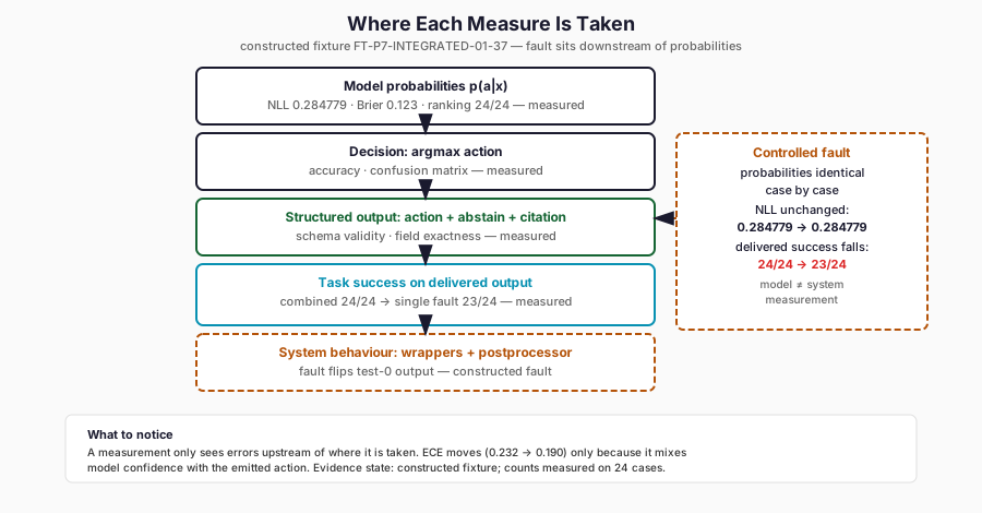
The figure names the boundary each measure belongs to. It is conceptual, drawn from the constructed fixture: probabilities are identical case by case across the fault, so NLL stays at 0.284779 while delivered task success falls from 24/24 to 23/24.
    flowchart LR
    P[model probabilities<br/>NLL, Brier, ranking] --> D[emitted action<br/>accuracy, ECE input]
    D --> S[structured output<br/>schema, fields]
    S --> T[task success<br/>action + abstain + citation]
    P -. fault downstream .-> F[postprocessor flips test-0]
    F --> T
Counting outcomes
For a classification into K classes, the confusion matrix C has one row for
each true class and one column for each predicted class. C[g, p] counts the cases
with gold label g and prediction p. The implementation adds one extra column,
INVALID, for responses that fail the schema. An invalid response therefore
stays in the denominator. It cannot vanish from the evaluation by failing to
parse.
For a class c, define true positives, false positives and false negatives:
Macro-F1 is the unweighted mean of F₁ over the declared classes. It is null if any class F₁ is undefined, which happens only when a class is absent from both gold and predictions. Micro aggregation pools the counts first. For a single-label problem with every case in the denominator, micro-F1 equals the diagonal of C divided by n, which is accuracy. Under the implementation’s convention an invalid output contributes one false positive and one false negative to the pooled count, so the identity still holds.
Macro and micro answer different questions. Micro weights each case equally, so a large class dominates it. Macro weights each class equally, so a failure confined to a small class shows through. Neither is the right answer in general. A report should give the per-class table and say which average it chose.
Selective prediction adds the option to decline (Geifman and El-Yaniv, 2017). Here declining means routing a case to review. Two quantities matter:
Probability quality is measured by two proper scoring rules, which are optimised in expectation by reporting the true conditional distribution (Gneiting and Raftery, 2007). For a case with gold class g and predicted probabilities p:
Expected calibration error asks whether stated confidence matches observed correctness (Naeini, Cooper and Hauskrecht, 2015; Guo et al., 2017). Group cases into M bins by confidence, here the maximum probability. For each bin B_m, compare mean confidence with the fraction correct:
Finally, ranking accuracy counts cases where the gold class has strictly the highest probability. Ties do not pass.
A four-case example by hand
The evaluation’s unit tests include a fixture small enough to compute by hand. It is a mathematical example, not experimental evidence. There are four cases:
| Case | Gold | Output | Probabilities (complete, refuse, review) |
|---|---|---|---|
| 1 | complete | complete | (0.8, 0.1, 0.1) |
| 2 | refuse | complete | (0.6, 0.3, 0.1) |
| 3 | review | review, abstain | (0.1, 0.2, 0.7) |
| 4 | complete | invalid | (0.2, 0.5, 0.3) |
The confusion matrix has C[complete, complete] = 1, C[complete, INVALID] = 1,
C[refuse, complete] = 1 and C[review, review] = 1. For complete, TP = 1,
FP = 1 (case 2) and FN = 1 (case 4), so F₁ = 2/4 = 0.5. For refuse, TP = FP = 0
and FN = 1, so precision is undefined and F₁ = 0. For review, F₁ = 1. Macro-F1 is
(0.5 + 0 + 1)/3 = 0.5, and accuracy and micro-F1 are both 2/4. Coverage counts the
valid, non-abstaining cases 1 and 2, giving 2/4, and selective accuracy is 1/2.
The Brier terms are 0.06, 0.86, 0.14 and 0.98, with mean 0.51. Case 4 keeps its
probabilities in the calibration measures even though its output was invalid.
What the experiment measured
All seven systems were run on the 24 test cases of each data seed. The counts below come from the raw per-case outputs, not from a summary. The authoring cross-check recomputed them independently, without importing the evaluation code. It reconstructed every probability vector from the constructed weights, and the largest disagreement with the recorded values was below 10⁻¹².
| System | Task success | Coverage | Abstentions | Brier | NLL | ECE |
|---|---|---|---|---|---|---|
| Base | 8/24 | 24/24 | 0/24 | 0.899 | 1.447 | 0.313 |
| Adapter A | 12/24 | 24/24 | 0/24 | 0.739 | 1.217 | 0.334 |
| Adapter B | 20/24 | 12/24 | 12/24 | 0.259 | 0.474 | 0.075 |
| Combined | 24/24 | 12/24 | 12/24 | 0.123 | 0.284779 | 0.232 |
| Weak-B control | 16/24 | 20/24 | 4/24 | 0.437 | 0.714 | 0.287 |
| Rule baseline (oracle) | 24/24 | 12/24 | 12/24 | 0.000 | 0.000 | 0.000 |
| Single fault | 23/24 | 12/24 | 12/24 | 0.123 | 0.284779 | 0.190 |
The aggregate rows are identical at seeds 37 and 38. That is expected rather than reassuring. Both seeds contain four copies of each pattern, and every model is a deterministic function of the pattern.
The counts follow from the weights. The base completes everything, so it succeeds only on the 8 read and copy cases. Adapter A adds the 4 certain erases but refuses the 4 uncertain erases, which needed review: 12/24. Adapter B routes all 12 review cases correctly but still completes the 4 certain erases: 20/24. The combined system gets all 24. The weak-B control, at weight 0.3, shifts only 0.9 units of score towards review. That is enough for the unknown-operation cases and not for the uncertain read or erase cases: 16/24.
The per-class table for the base system shows why one score is not enough:
| Class | Support | Precision | Recall | F₁ |
|---|---|---|---|---|
| complete | 8 | 8/24 | 8/8 | 0.5 |
| refuse | 4 | undefined (0/0) | 0/4 | 0 |
| review | 12 | undefined (0/0) | 0/12 | 0 |
Its macro-F1 is 0.167 and its accuracy is 8/24. Both numbers are low. Neither says, as the table does, that the model never refuses and never asks for review.
The combined system is perfect on task success and still has an ECE of 0.232. It is underconfident, not wrong. Its 8 read and copy answers carry a confidence of only 0.576 each, because for those inputs the winning score exceeds the other two by just one unit. Calibration and correctness are different properties, and a calibration diagnostic can flag a system that never errs.
The controlled fault
Now compare the combined system with the single-fault system. Both rest on the same model. Every probability vector is identical, case by case, in the raw records. The scoring rules see nothing:
| Measure | Combined | Single fault | Boundary |
|---|---|---|---|
| Mean NLL | 0.284779 | 0.284779 | model probabilities |
| Mean Brier | 0.123 | 0.123 | model probabilities |
| Ranking accuracy | 24/24 | 24/24 | model probabilities |
| ECE | 0.232 | 0.190 | probabilities and emitted action |
| Action accuracy | 24/24 | 23/24 | emitted action |
| Task success | 24/24 | 23/24 | delivered structured output |
The NLL can be derived by hand. A read or copy request has scores (1, 0, 0) under the combined weights, so the gold probability is e/(e + 2) and its NLL is 0.551445. The four other patterns have smaller losses: 0.169846 for a certain erase, 0.065884 for an uncertain read, 0.315072 for an uncertain erase and 0.054985 for an unknown operation. Each pattern appears four times. The mean of the six pattern losses is 0.284779.
The fault itself depends on the seed, because test-0 holds a different pattern
at each seed. At seed 37 it is a copy request whose correct action is complete.
The postprocessor turns it into an unwarranted refusal. At seed 38 it is a
certain erase whose correct action is refuse. The postprocessor turns it into
complete, so the system executes a disallowed operation. The two faults differ
in kind, and macro-F1 shows it: 0.941 at seed 37 and 0.933 at seed 38. Task
success shows 23/24 at both.
Why can NLL not see the fault? Negative log-likelihood is a function of the model’s probability for the gold class and of nothing else. The fault happens after the probabilities are produced. The probabilities are recorded and the output is rewritten, so the two quantities are measured at different boundaries. A measurement can only detect errors introduced upstream of the point where it is taken.
ECE changes for a subtler reason. Its correctness indicator uses the emitted action, and the faulty case now counts as wrong in its confidence bin. That does not make ECE a fault detector. It mixes model confidence with system output and can move for reasons unrelated to either alone. The clean lesson is the structural one: model evaluation and end-to-end system evaluation are different measurements. A model-side report, however careful, cannot certify the delivered system.
Negative controls
The evaluation machinery is itself tested by controls meant to fail.
- An invalid output stays in the denominator. Chapter 39 runs a control whose every response violates the schema. It scores 0/24 on task success and on schema validity.
- A wrong citation with the right action fails task success. A unit test changes one citation and observes action accuracy 1 and task success 0.
- Missing classes produce nulls. On a one-case fixture, macro-F1, abstention correctness and the recall of an absent class are all reported as null.
- A forged schema flag is refused. If a record claims that an invalid output
was valid, the evaluator raises
SCHEMA_WITNESSinstead of scoring it. - Malformed probability vectors, of the wrong length, not summing to one or containing NaN, are refused.
These are tests of the software, not observations about any model.
What the experiment does and does not show
It shows that the evaluation code computes what its definitions say. Every count was recomputed from raw outputs, and every probability from the weights. It shows that a postprocessor fault can lower delivered task success while every probability-based model measurement stays fixed. And it shows that an underconfident system can be perfect, and that a model can be locally accurate on one class while useless on two others.
It does not show that any adapter learned anything. The adapters were written down. It does not show that the evaluation would detect errors in a real language model’s free-text output. The task has six patterns and a structured response. It does not establish production-level coverage, because 24 cases drawn from six patterns are a check of software behaviour, not a sample from a population of requests. And the perfect rule baseline means that, on this task, no model is needed at all. Every adapter result has to be read against that oracle.
Practical lessons
- Define task success on the delivered output, against the full contract. Report action accuracy and probability measures as well, but name their boundaries.
- Keep every case in its denominator. Invalid outputs, abstentions and missing classes each need explicit treatment, and an undefined ratio should be reported as undefined.
- Report per-class results before averages. Say whether an average is macro or micro.
- Pair a proper scoring rule with any binned calibration diagnostic, and state the binning.
- Include an oracle or rule baseline when one exists, and say why it scores what it scores.
- Treat a postprocessor, a parser or a serving wrapper as part of the system under test. Model-side metrics cannot see faults downstream of the model.
Limitations
The task is synthetic, finite and benign, with six repeating patterns and 24 test
cases per data seed. The adapters are constructed, not trained. The two data
seeds produce identical aggregates because they contain the same patterns.
Groundedness means citing the declared policy digest and nothing more.
Calibration is computed with five declared bins on 24 cases, and its values are
coarse. The single-fault system is a deliberate controlled fault, not an observed
production bug. The records are engineering-stage evidence:
AUTHENTICATED_EXECUTION = NOT_ESTABLISHED, and local hashes establish
consistency with pinned files, not independent attestation that the runs
happened as described.
FineTuneLab
The task contract, policies, fixture and label authority live in
ftlab.delivery.task. The constructed base and adapters, the composition
arithmetic and the rule baseline are in ftlab.delivery.composition. The
evaluator in ftlab.delivery.evaluation seals each evaluation with its contract,
policy, label authority, dataset, model and adapter identities. It also checks
recorded schema flags against the actual output structure. The experiment is
ch37 in ftlab.delivery.experiments.
Where this leads
The combined system scored 24/24 and the base system 8/24. The difference of 16/24 is arithmetically certain. Whether it supports any wider conclusion depends on how the 24 cases were sampled, on which cases are correlated with which, and on what else changed between the two systems. Chapter 38, Statistical Confidence and Ablation, puts an interval around that difference. It then shows that the interval’s width depends on things a single score never reveals.
Further Reading
- Tilmann Gneiting and Adrian E. Raftery, “Strictly Proper Scoring Rules, Prediction, and Estimation” (2007). Read the source. The reference theory behind proper scoring rules, explaining why NLL and Brier score reward honest probabilities while binned diagnostics such as ECE cannot.
- Chuan Guo et al., “On Calibration of Modern Neural Networks” (2017). Read the source. The standard modern calibration study, supporting the chapter’s finding that a system can be perfectly successful yet miscalibrated.
- Yonatan Geifman and Ran El-Yaniv, “Selective Classification for Deep Neural Networks” (2017). Read the source. The framework behind coverage, selective accuracy and abstention accounting, with undefined ratios kept undefined.