Beyond Conventional LoRA
Classify IA3, prompt tuning, prefix tuning, DoRA and AdaLoRA by what each changes, derive the IA3 and soft-prompt mechanisms actually implemented, and keep unrun methods labelled as literature.
Parameter-efficient fine-tuning libraries offer a menu: LoRA, IA3, DoRA, AdaLoRA, prompt tuning, prefix tuning and more. The menu presentation suggests that these are interchangeable settings of one idea, to be swept like a learning rate. They are not. Each method restricts the adaptation in a different place, and the place determines what can be learned, what must be stored, whether the result can be merged into the base, and how the method interacts with context length and checkpoints.
Chapter 22 derived LoRA as an additive low-rank change to a weight matrix. This chapter begins from the opposite question: if not an additive low-rank weight change, then what? We classify the main alternatives by the object they modify, derive the two mechanisms this book implements and tests, and describe the others from their primary sources while marking them clearly as unrun.
The results below have also been executed in the pinned Docker CPU environment as FT-P5-INTEGRATED-02-26, using the repaired Part IV foundation and local FineTuneLab 0.12.0. The integrated evidence map records source, configuration, environment and artifact hashes for each claim. Earlier staging and authoring comparisons remain historical provenance; they are not independent acceptance. No pretrained-model operation is authorised by these runs.
Classify by the object being changed
Write a frozen linear map as Y = XW^T + b with the book’s row-batch convention from Chapter 22. An adaptation method must change something in the computation. The useful classification asks what:
| Method | Object changed | Trainable state | Starts as identity? |
|---|---|---|---|
| LoRA | Weight, additively | Factors A[r, d_in], B[d_out, r] | Yes, B = 0 |
| IA3 | Activations, multiplicatively | One vector per targeted activation | Yes, scales = 1 |
| DoRA | Weight, decomposed into magnitude and direction | Magnitude vector plus LoRA factors on direction | Yes, by initialisation |
| AdaLoRA | Weight, additively, with adaptive rank | SVD-form factors plus importance state | Yes, singular values start at zero |
| Prompt tuning | The input sequence | p virtual embeddings | No, by construction |
| Prefix tuning | Every layer’s attention memory | Prefix activations per layer | No, by construction |
Two families are already visible. LoRA, DoRA and AdaLoRA change weights and can, after training, be folded into a new weight. Prompt and prefix tuning change the sequence the frozen network sees; nothing is folded, and the extra positions cost context and memory at every inference. IA3 sits between: it multiplies activations, which turns out to be equivalent to scaling rows or columns of a weight, so it too can be folded.
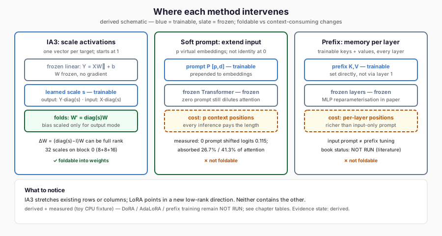
The figure contrasts the three implemented mechanisms by the object each changes. Notice that only weight and scale changes fold back into the base, while sequence changes consume context at every inference.
The final column matters in practice. A method that starts as an exact identity leaves the base model’s behaviour unchanged at step zero, so any later change is attributable to training. A method that cannot start as an identity alters the model before learning begins. We will measure one such alteration below.
Derive IA3 as a learned diagonal
The IA3 method, from Liu and colleagues, multiplies selected activations element-wise by learned vectors initialised to ones. In their Transformer formulation the vectors rescale the attention keys, the attention values, and the intermediate activation of the feed-forward network after its nonlinearity.
Consider a single linear layer and two ways to place a scale vector.
Output scaling multiplies the layer’s output:
With G = dL/dY, define Z = XW^T + 1b^T for output scaling. The gradients are
The folded form also clarifies how IA3 restricts the update. The effective weight change for output scaling is
Work through the scalar reference
The implementation checks its layer against a pure-Python loop that shares no tensor code with it. Take
For input scaling with s = (0.5, 2, -1), the first row of X diag(s) is (0.5, 0, 2), giving outputs (-1.25, 0.5); the second row gives (5, -0.5). The gradient is (1.5, 19.5, -12.5).
In FP64, the module’s forward outputs and scale gradients match these scalar values with zero error in both modes, and no gradient is created for the frozen weight. A separate check against the IA3 linear layer in PEFT 0.18.0, configured with the same weight, bias, scale and placement, also agreed with zero forward and gradient error. That parity covers matched standalone layers only; it says nothing about how PEFT chooses target modules in a full model.
An authoring check confirms the folding argument numerically: building W’ and b' explicitly reproduces both modes’ outputs exactly, and the resulting ΔW has rank 2, the full rank of this 2 × 3 matrix.
Place IA3 inside the Transformer
Our causal Transformer fuses the query, key and value projections into one linear layer of width 3d. IA3 must scale keys and values but not queries, so the implementation splits the fused output into thirds and multiplies only the second and third:
Placement after the nonlinearity is not a cosmetic detail. Scaling before the
nonlinearity would be output scaling on up, giving γ(s ⊙ z) rather than
s ⊙ γ(z). For GELU with s = 2 and z = 1, the first is GELU(2) ≈ 1.9545 while the
second is 2 · GELU(1) ≈ 1.6827. A method label that says “IA3 on the MLP”
without stating the placement does not identify a function.
On the chapter’s model (width d = 8, MLP width f = 16), IA3 on block 0 has d + d + f = 8 + 8 + 16 = 32 scales. The rank-2 LoRA adapter from Chapter 25 also had 32 parameters. Equal counts are a coincidence of these dimensions, not evidence that the methods are comparable.
Measure the IA3 mechanism
The experiment attaches IA3 to block 0 of the same seed-37 model used in Chapter 25. Before training, the logits with all scales at one differed from the unadapted model’s logits by exactly zero: the identity initialisation holds. Four full-batch AdamW updates at learning rate 0.02 on the same two training rows then gave losses of
5.445624, 5.442575, 5.439539, 5.436520.
A frozen-state witness confirmed that every base parameter and buffer was bitwise unchanged after each update. The scales were saved with a manifest binding the method, the exact targets and their dimensions, the frozen-base digest and the experiment configuration. Reloading them into a fresh model gave zero maximum logit error.
The loss decrease is small, as Chapter 25 would predict for 32 parameters, four steps and a learning rate chosen for a different purpose. This is a mechanism check, not a comparison with LoRA. Nothing here says which method is better at anything.
Derive why a zero soft prompt is not a no-op
Prompt tuning, introduced by Lester, Al-Rfou and Constant, prepends p trainable vectors to the embedded input sequence of a frozen model. The paper reports that the method becomes competitive with full model tuning as model scale grows into the billions of parameters; that claim concerns pretrained models far outside this book’s experiments.
Here we implement only the mechanism, on a deliberately tiny frozen network: an eight-token embedding of width 4, one causal self-attention layer with a single head, and a two-way classifier reading the last position. The prompt is a trainable 2 × 4 matrix, initialised to zeros.
Initialising a soft prompt to zeros sounds as if it should leave the model unchanged. It does not, and the reason is worth deriving.
In PyTorch’s multi-head attention, the input projection biases are initialised to zero. A zero prompt embedding therefore produces zero keys and zero values. At the final query position, the attention score against each prompt key is q · 0 / √d_k = 0, so each prompt position receives softmax weight proportional to exp(0) = 1. The real positions’ weights become
The measured outputs agree. For two input sequences, the zero-prompt logits differed from the no-prompt logits by up to 0.114830. An authoring check recomputed both outputs by explicit softmax, using the module’s weights, and matched the module to within 3 × 10⁻⁸. It found that the zero prompt absorbed 26.7% and 41.3% of the final position’s attention in the two sequences.
The gradient with respect to the prompt was non-zero, with norm 0.038043 under a sum-of-squares loss, and one SGD step changed only the prompt: the frozen witness held. The mechanism trains, but it never starts from an exact identity. Any comparison involving prompt tuning must report the zero-step change as part of the method. This toy omits positional encoding, so permuting its prompt rows leaves the example’s output unchanged; it does not establish that prompt order is irrelevant in a model with positional information.
Prefix tuning is not an input prompt
Prefix tuning, by Li and Liang, is often described as the same idea. It is not. Prefix tuning prepends trainable activations at every layer, so each layer’s attention can read prefix keys and values that are free parameters rather than functions of earlier layers. The authors also reparameterise the prefix through a small network during training, reporting that direct optimisation was less stable, and keep only the resulting prefix afterwards.
The distinction can be stated precisely. With an input soft prompt, the prompt’s representation at layer two is computed by the frozen first layer from the layer one prompt. It is constrained to whatever the frozen network can produce from some input vector. With prefix tuning, the layer-two prefix keys and values are set directly. The family of reachable attention memories is larger.
This book has not implemented prefix tuning. The input prompt above must not be reported as a prefix-tuning result, and the implementation records prefix tuning as unrun for exactly that reason.
DoRA decomposes a weight before adapting it
DoRA, from Liu and colleagues, separates a weight’s magnitude from its direction and adapts the direction with low-rank factors. Its notation and the released implementations need to be stated separately.
In the paper, W and V have shape [d, k], the magnitude m has shape [1, k], and ‖V‖_c is the vector of norms across the columns. Its decomposition is
These are not automatically the same operation. On the non-square fixture
The paper also proposes treating the norm denominator as constant during backpropagation, which changes the direction gradient despite an unchanged forward value. A faithful executable comparison would therefore have to pin both the norm axis and the gradient treatment. This book has not established that parity. DoRA is therefore described here from its source and left unrun. The small norm fixture checks two reductions, not DoRA training or performance.
AdaLoRA makes rank a learned budget
AdaLoRA, from Zhang and colleagues, keeps an additive update but writes it in a singular-value-decomposition form, PΛQ: two factor matrices and a diagonal of singular values. The diagonal starts at zero, so the update starts as an identity, and a penalty pushes P and Q towards orthogonality so that the diagonal behaves like singular values. During training, it scores the importance of each singular component and prunes the least important, so the rank budget migrates towards the weight matrices that seem to need it.
The consequence for engineering is that the shape of the trainable state can change during training. Optimiser state, checkpoint contents and the rank reported in a result all depend on when they are read. Chapter 30’s requirement that a checkpoint record complete training state applies with extra force: a resumed AdaLoRA run must restore the current budget schedule and masks, not only the factors.
AdaLoRA is unrun in this book. The description above is literature-supported only.
The methods are not interchangeable
The algebra produces practical differences that no hyperparameter sweep can erase.
| Question | LoRA | IA3 | DoRA | AdaLoRA | Prompt | Prefix |
|---|---|---|---|---|---|---|
| Can it be folded into the weights after training? | Yes | Yes | Yes | Yes | No | No |
| Does it consume context positions? | No | No | No | No | Yes, p per sequence | Yes, per layer |
| Is the update low-rank? | Yes, ≤ r | No, diagonal | Direction yes, magnitude no | Yes, rank varies | Not a weight update | Not a weight update |
| Exact identity at step zero? | Yes | Yes | Yes | Yes | No | No |
| Implemented and tested here | Chapter 22 | Yes, tiny CPU | No | No | Mechanism only | No |
A comparison that sweeps “method” as one axis mixes all of these differences with whatever the experiment intends to measure. If a prompt-tuning run underperforms, is it the method, the lost context, or the zero-step dilution? If IA3 underperforms LoRA at equal parameter count, is it the diagonal restriction, the placement, or a learning rate chosen for LoRA? The comparison must hold the non-method differences fixed or report them, which is the same discipline as Chapter 23 applied to a harder axis.
Failure modes the tests guard against
The implementation’s negative tests describe the ways an alternative method can be mislabelled:
- IA3 attached to a module whose shape does not match the reviewed fused layout, attached twice, or attached to an already adapted layer;
- a trainable parameter outside the declared scales, or a missing scale;
- a base parameter that changed during training;
- a checkpoint relabelled as a different method and re-sealed, which the method-and-layout binding rejects even though its digest is internally consistent;
- scales loaded into a model with a different frozen base or a different precision;
- a soft-prompt configuration or token range outside the declared bounds.
One test deserves a sentence. Re-sealing a relabelled checkpoint produces a manifest whose digest is valid. Integrity alone cannot detect the change. The load is refused because the manifest’s method and layout must equal the receiving model’s actual targets, which are computed from the live module tree.
Limitations
The IA3 run uses a random tiny model, two training rows, four updates and CPU FP32. The soft-prompt run uses a separate frozen toy classifier and one SGD step. Neither experiment says anything about task quality, data efficiency or the relative merits of the methods. DoRA, AdaLoRA and prefix tuning have no executed evidence in this book; their descriptions rest on their papers. Real-model adaptation of any kind remains blocked by the acquisition gate.
The IA3 and soft-prompt evidence was recorded in the engineering staging environment and reproduced in a separate authoring container against the repaired Part IV package. The identity error, reload error, scale count, IA3 losses and all scalar-reference values matched exactly. The soft-prompt outputs and gradient norm agreed to within about 3 × 10⁻⁸, a floating-point difference between two builds of the same library.
FineTuneLab
The mechanisms live in the module ftlab.advanced.alternatives,
integrated with the repaired Part IV package. IA3Linear implements
input and output scaling with explicit precision handling; IA3QKV scales only
keys and values in the fused projection; attach_ia3 targets declared blocks;
SoftPrompt is the input-prompt mechanism; save_method_state and
load_method_state bind scales to method, layout, frozen base and experiment;
mathematical_reference is the scalar check. The module records DoRA, AdaLoRA and
prefix tuning as not run. It is included in the locally verified 0.12.0 wheel, which has not been published.
Where this leads
Chapters 25 and 26 have asked which parameters move and how the movement is parameterised. Neither asked what the movement is aimed at. The next chapter, Continued Pretraining Versus Instruction Tuning, keeps the parameterisation fixed and changes the objective: learning a domain’s token distribution, learning an instruction-to-response mapping, and answering from information that changes after training.
Further Reading
- Haokun Liu et al., “Few-Shot Parameter-Efficient Fine-Tuning is Better and Cheaper than In-Context Learning” (2022). Read the source. Introduces (IA)3, which scales activations by learned vectors, outperforming in-context learning within the T-Few recipe. Read it for the rescaling-vector placements the chapter folds into equivalent weights.
- Brian Lester, Rami Al-Rfou and Noah Constant, “The Power of Scale for Parameter-Efficient Prompt Tuning” (2021). Read the source. Prepends trainable soft prompts to a frozen model, closing the gap to full tuning at billion-parameter scale. Read it for the mechanism whose zero-initialised dilution the chapter derives and measures.
- Xiang Lisa Li and Percy Liang, “Prefix-Tuning: Optimizing Continuous Prompts for Generation” (2021). Read the source. Prepends trainable prefixes at every layer and matches fine-tuning with 0.1% of parameters. Read it to see why per-layer prefixes reach memories an input-only prompt cannot.