Alternatives to DPO
Derive ORPO, SimPO and KTO from the choices DPO makes, fix a real numerical defect in the odds calculation, and compare the objectives on one starting policy where SimPO's own objective improves while held-out agreement falls to 1/4.
Chapter 32’s objective made four choices. It scored a response by its summed log probability. It measured the policy’s preference relative to a frozen reference. It linked preference to score through the Bradley–Terry logistic function. And it consumed pairs: one preferred and one rejected response for the same prompt.
Each choice can be made differently, and a family of methods has done so. This chapter derives three of them from the choices they change:
- ORPO keeps pairs but drops the reference, normalises by length, replaces log probability with log odds, and adds an ordinary supervised term.
- SimPO keeps pairs and the logistic link but drops the reference, normalises by length and demands a target margin.
- KTO drops pairs altogether and learns from responses labelled simply desirable or undesirable.
The chapter then runs DPO, ORPO and SimPO from the same starting policy on the same data. KTO’s scalar loss was implemented and checked against independent arithmetic, but a full KTO training loop and its minibatch reference-point estimator were not executed, so it has no experimental results here.
The measured results were recorded as FT-P6-INTEGRATED-02-33-s37 and FT-P6-INTEGRATED-02-33-s38 on a randomly initialised policy. The integrated runs are bitwise-identical to the preserved historical records FT-P6-CODEX-03-33-s37/s38 and are not a ranking of these methods for real fine-tuning.
Two ways to score a response
Write ℓ(y) = log π_θ(y | x) for the summed log probability of a response with |y| target tokens, as in Chapter 32, and
The choice can reverse a comparison. Suppose a preferred response has two tokens with summed log probability −3 and a rejected response has six tokens summing to −6. By sum, the preferred response is more probable by 3 nats. By mean, it scores −1.5 against −1.0, and the rejected response is preferred by 0.5 nats per token. Neither number is “the” preference; they answer different questions. A sum asks how probable the whole response is. A mean asks how probable a typical token in it is, and stops a method rewarding a response merely for being short.
Both ORPO and SimPO use the mean. In the experiment below every candidate has exactly two target tokens, so ℓ̄ = ℓ/2 and the distinction changes no ordering; it only rescales.
ORPO: supervision plus an odds ratio
Hong, Lee and Thorne’s ORPO: Monolithic Preference Optimization without Reference Model folds preference alignment into supervised fine-tuning. It treats exp(ℓ̄(y)) as a length-normalised probability P, defines the odds P/(1 − P), and contrasts the odds of the preferred and rejected responses. In log form, for a mean log probability a < 0,
Log odds behave differently from log probabilities near certainty. Their derivative is
A worked example. Take mean log probabilities a = −1 for the preferred response and b = −2 for the rejected one. Their plain difference is 1. Their log odds are about −0.541325 and −1.854587, so the log-odds margin is about 1.313262. With λ = 0.1 the loss is 1 + 0.1 × log(1 + exp(−1.313262)) ≈ 1.023818. The gradient with respect to a is −1 from the supervised term plus about −0.033529 from the odds-ratio term, the latter being −λ σ(−1.313262)/(1 − exp(−1)). The gradient with respect to b is about +0.024511. The supervised term dominates by a factor of about thirty.
A numerical defect worth understanding
Computing log(1 − e^a) looks harmless. It is not. When a is very close to
zero, e^a is very close to one, and subtracting it from one loses almost every
significant digit. In FP32, exp(−10⁻⁸) rounds to exactly 1, so the naive
expression returns log(0) = −∞. The stable form uses the library function
expm1(a), which computes e^a − 1 accurately for small a, and writes
An earlier engineering revision tried to have the best of both regimes with
an elementwise switch: use log1p(-exp(a)) when a < −log 2 and
log(-expm1(a)) otherwise, selected with torch.where. The forward value was
correct everywhere. The gradient was not. torch.where evaluates both
branches for every element and then selects. At a = −10⁻⁸ the unused branch
evaluates log1p(−1) = −∞ and its derivative is −∞. In the backward pass the
unused branch receives a zero gradient from the selection, and zero times
infinity is NaN. The NaN propagates into the selected element’s gradient.
Reproducing the old expression in FP32 confirms each step: at a = −10⁻⁸ the
old form returns the correct value −18.420681 and a NaN gradient, while the
single log(-expm1(a)) form returns the same value and a gradient of
−1.0 × 10⁸, against an exact FP64 derivative of about −9.99999995 × 10⁷. At
a = −0.5 and a = −2 the two forms agree in both value and gradient.
The engineering batch replaced the switch with the single expression and preserved the corrected source under the historical namespace FT-P6-CODEX-03; the integrated namespace FT-P6-INTEGRATED-02 replays it bitwise-identically. Results from the earlier namespaces were not rewritten and are not used in this book. The lesson is general: when a function is assembled from branches, check the gradient of every branch at every input the selection could see, not only the value of the branch that was selected.
SimPO: a reference-free margin
Meng, Xia and Chen’s SimPO: Simple Preference Optimization with a Reference-Free Reward keeps DPO’s logistic link but changes the score. Its implicit reward is the length-normalised log probability scaled by β, and it asks the preferred response to win by at least a target margin γ:
Two properties follow directly from the formula.
First, γ keeps the loss pushing after the pair is ordered correctly. A pair with zero mean-log-probability gap has margin −γ, loss log(1 + exp(γ)) and gradient weight σ(γ). With γ = 0.5 that is a loss of about 0.974077 and a weight of about 0.622459, greater than the 0.5 a tie receives in DPO.
Second, without a reference, SimPO sees the policy’s absolute preference. DPO, by construction, sees only how far the policy has moved from the reference. A preference the policy inherited at initialisation is invisible to DPO and fully visible to SimPO. This difference turns out to explain the experiment.
A worked example. With ℓ̄(y_w) = −1, ℓ̄(y_l) = −2, β = 2 and γ = 0.5, the margin is 2 × 1 − 0.5 = 1.5 and the loss is log(1 + exp(−1.5)) ≈ 0.201413. The gradient with respect to ℓ̄(y_w) is −β σ(−1.5) ≈ −0.364851, and with respect to ℓ̄(y_l) it is the same magnitude with the opposite sign.
KTO: desirable and undesirable responses
Ethayarajh and colleagues’ KTO: Model Alignment as Prospect Theoretic Optimization starts from a different kind of data. Each example is a single response labelled desirable or undesirable. Nothing pairs it with an alternative for the same prompt. Such labels are often cheaper to collect, for example as thumbs-up and thumbs-down feedback.
KTO keeps DPO’s implicit reward r_θ = log π_θ(y|x) − log π_ref(y|x) and compares it with a reference point z₀, defined as the KL divergence of the policy from the reference. The paper’s value function is λ_D σ(β(r_θ − z₀)) for desirable responses and λ_U σ(β(z₀ − r_θ)) for undesirable ones, with class weights λ_D and λ_U, and the loss for an example is its class weight minus its value. Simplifying with 1 − σ(z) = σ(−z):
In practice the paper does not compute z₀ exactly. It estimates it from mismatched prompt–response pairs within a microbatch, clamps the estimate at zero, and does not backpropagate through it; the authors describe it as a biased surrogate that is easy to calculate.
The book’s implementation is narrower, and the boundary matters. The scalar loss is implemented with z₀ supplied explicitly as a detached, non-negative number, either an exact KL on a finite support or a fixed value. For r_θ = 1, z₀ = 0.1, β = 0.2 and unit weights, the desirable loss is σ(−0.18) ≈ 0.455121 and the undesirable loss for the same inputs is about 0.544879; both values were checked against independent arithmetic. No KTO model was trained, and the microbatch estimator was not implemented. KTO therefore appears in this chapter’s mathematics and not in its results.
Compare the objectives
| Property | DPO | ORPO | SimPO | KTO (book scalar) |
|---|---|---|---|---|
| Data | Strict pairs | Strict pairs | Strict pairs | Single responses, desirable or undesirable |
| Reference policy | Required, frozen | None | None | Required, plus reference point z₀ |
| Score | Summed log probability | Mean log probability, as log odds | Mean log probability | Summed log ratio |
| Supervised term | None | NLL of preferred response | None | None |
| Link | −log σ | −log σ on log-odds ratio | −log σ with target margin | Bounded σ with class weights |
| Executed here | Yes | Yes | Yes | Scalar checks only |
The losses have different units and different minima. ORPO’s includes a negative log-likelihood that is large for an untrained model; SimPO’s includes a margin offset; DPO’s starts at exactly log 2. Comparing their numeric values across methods says nothing. Each objective can be compared only with itself, before and after training.
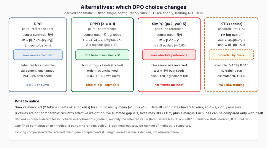
The figure places the four objectives side by side by reference use, score and link. Notice that only ORPO adds a supervised term, only SimPO demands a margin, and KTO here is a scalar check with no training run.
The experiment
For each seed, all three methods start from the same randomly initialised 5,064-parameter policy, with an identical state digest, and use the same eight training pairs from Chapter 31, cycled four times over 32 updates with AdamW at learning rate 0.01. Method-specific settings are fixed in advance: DPO with β = 0.2 on summed log probabilities; ORPO with λ = 0.1 and SimPO with β = 2 and γ = 0.5, both on mean log probabilities. The DPO run is the same run as Chapter 32’s clean condition; its final policy digest is identical.
Common inputs and seeds do not make the methods’ hyperparameters comparable. β = 0.2 on a sum and β = 2 on a mean of two tokens are not “the same strength”: on these two-token responses SimPO’s effective coefficient on the summed log-probability gap is 1, five times DPO’s 0.2, and it adds a margin. No setting was tuned for any method. The comparison shows how three fixed configurations moved one tiny policy; it does not rank the methods.
Held-out agreement is defined as in Chapter 32: the policy’s own teacher-forced log probability of the preferred candidate must exceed that of the rejected one.
| Seed | Method | Train before → after | Validation before → after | Test before → after |
|---|---|---|---|---|
| 37 | DPO | 4/8 → 4/8 | 2/4 → 2/4 | 2/4 → 2/4 |
| 37 | ORPO | 4/8 → 4/8 | 2/4 → 2/4 | 2/4 → 2/4 |
| 37 | SimPO | 4/8 → 7/8 | 2/4 → 2/4 | 2/4 → 1/4 |
| 38 | DPO | 4/8 → 4/8 | 1/4 → 1/4 | 3/4 → 3/4 |
| 38 | ORPO | 4/8 → 4/8 | 1/4 → 1/4 | 3/4 → 3/4 |
| 38 | SimPO | 4/8 → 4/8 | 1/4 → 3/4 | 3/4 → 1/4 |
Each method’s own objective, recomputed over all eight training pairs from the stored log probabilities before and after training, decreased at both seeds:
| Seed | DPO | ORPO | SimPO |
|---|---|---|---|
| 37 | 0.693147 → 0.692538 | 5.829636 → 1.117235 | 1.081520 → 0.969174 |
| 38 | 0.693147 → 0.690534 | 5.873788 → 1.255183 | 1.162003 → 0.958954 |
SimPO’s training objective improved at both seeds, and its held-out agreement fell to 1/4 at both seeds.
Read what each method did
The starting policy, as Chapter 32 found, prefers the string 1 over 0 on
every prompt by roughly one nat at seed 37 and 1.3 to 1.4 nats at seed 38.
Every result in the table follows from what each objective did to that
prompt-blind preference.
DPO measures preference relative to the reference, which is the starting policy. At the first update every margin is zero and every pair receives the same gradient weight, 0.5. Balanced training labels then push the string preference equally in both directions. The inherited bias is not an error in DPO’s eyes, so DPO barely touches it.
ORPO mostly did supervised learning. Its supervised term raises the probability of whichever string is preferred, and with balanced labels that means both strings. On the test prompts the summed log probability of each candidate rose by between 9.1 and 9.6 nats: the policy learned that an answer here is a single digit followed by end-of-sequence. That is most of the objective’s fall from about 5.8 at seed 37 and 5.9 at seed 38 to about 1.1 and 1.3. The odds-ratio term, at weight 0.1, changed the gap between the two strings only modestly, from about 0.97 to about 0.68 nats at seed 37 and from about 1.36 to between 1.51 and 1.60 nats at seed 38, without changing its sign on any prompt. The ordering of every pair, and so every count, stayed where it was.
SimPO sees the inherited preference as an error. Without a reference, a
pair that prefers 0 starts with a strongly negative margin and a pair that
prefers 1 with a positive one. Using a string gap of 0.97 nats over two
tokens, the starting margins are about −1.47 and +0.47, with gradient weights
of about 0.81 and 0.38. The push towards 0 is roughly twice the push towards
1, and the policy’s string bias collapses.
At seed 37 the gap between the strings fell to within 0.016 nats of zero on every test prompt. With the bias gone, the training pairs’ orderings were decided by small prompt-dependent differences, and seven of the eight training pairs came out in the labelled direction. Those differences did not carry over: one of four test pairs agreed, and the orderings that decided the count were separated by hundredths of a nat.
At seed 38 SimPO overshot. The preference reversed to favour 0 on every
prompt in every split, by between 0.06 and 0.21 nats. The policy was again
prompt-blind, now in the other direction, and its agreement counts follow
mechanically from the labels. One test pair prefers 0, so test agreement is
1/4. Three validation pairs prefer 0, so validation agreement rose from
1/4 to 3/4. Half the training pairs prefer 0, so training agreement stayed
at 4/8.
The SimPO result therefore deserves careful wording. It does not show that SimPO “learned the wrong rule”. At seed 38 it learned no rule; it replaced one string bias with a smaller opposite one, and the held-out count fell because of which labels the four test pairs happen to have. At seed 37 it removed the bias and left orderings too close to zero to mean anything. In both cases its own objective improved while held-out agreement fell, which is exactly the gap between optimisation and outcome that this part of the book is about.
What the comparison establishes
It establishes that three objectives started from one policy on one dataset can move that policy in visibly different ways: DPO left an inherited preference almost untouched; ORPO mainly learned the response format; SimPO removed, and at one seed reversed, the inherited preference. It establishes that ORPO’s log odds need a numerically careful implementation, and that an elementwise branch can poison gradients that its forward values conceal.
It does not establish that any method is better than another for fine-tuning. The configurations were not tuned, the effective strengths differ, the policy is random, the candidates are two single-character strings, the held-out set has four pairs and its label composition, not learning, determines most of the counts. A claim that SimPO harms generalisation, or that ORPO is inert, would need a pretrained starting policy, responses of varying length, matched optimisation budgets and far larger held-out sets.
Limitations
Only DPO, ORPO and SimPO were executed, each with one fixed configuration and 32 updates on eight pairs. KTO’s loss was validated as a scalar function with a supplied reference point; no KTO training loop or microbatch estimator was run. All candidates are equal in length, so the length-normalisation argument is derived, not observed. No trainer library was installed or compared, and no parity with any external implementation is claimed. Held-out agreement uses four pairs per seed and teacher-forced scoring of fixed strings.
FineTuneLab
The objectives live in ftlab.preferences.objectives. orpo takes mean log
probabilities, computes log odds through log_odds, which uses the single
log(-expm1(·)) expression and refuses non-negative inputs, and returns the
supervised and odds-ratio components separately. simpo takes mean log
probabilities and refuses a negative margin γ. kto takes per-example log
probabilities, frozen reference log probabilities, a Boolean desirable mask and
a detached non-negative scalar reference point, and applies the two class
weights explicitly without fabricating a missing class. sequence_logps
supplies summed or mean completion log probabilities. The comparison run is
offline_preference with method set to dpo, orpo or simpo, and the
FP32 regression that reproduces the earlier branch defect sits beside the
integration tests.
Where this leads
DPO, ORPO and SimPO all fold the notion of “better” into the policy’s own probabilities. The older route makes that notion an explicit object: a reward model that scores responses, which a separate optimiser then pursues. The next chapter builds both halves, a tiny reward model and a PPO-style optimiser, and finds that the reward model’s failures on this fixture are exactly predictable from a fact Chapter 31 recorded about the split.
Further Reading
- Jiwoo Hong, Noah Lee and James Thorne, “ORPO: Monolithic Preference Optimization without Reference Model” (2024). Read the source. Folds alignment into supervised tuning with an odds-ratio penalty and no reference model. Read it for the log-odds margin whose stable form the chapter adopts.
- Yu Meng, Mengzhou Xia and Danqi Chen, “SimPO: Simple Preference Optimization with a Reference-Free Reward” (2024). Read the source. Uses mean log-probability with a target margin and outperforms DPO without length exploitation. Read it for the absolute scoring that erased the chapter’s inherited bias.
- Kawin Ethayarajh et al., “KTO: Model Alignment as Prospect Theoretic Optimization” (2024). Read the source. Learns from unpaired desirable and undesirable responses. Read it for the binary-feedback setting the chapter formalises but does not train.