Scaling Beyond One GPU
Derive what data parallelism, ZeRO, FSDP, CPU offload and activation checkpointing change in per-device memory and communication, and validate a planning ledger without mistaking it for a measurement.
There are two different reasons to train on more than one device, and they are often confused. The first is time: one device could hold the training state but would take too long, so several devices each process part of every batch. The second is memory: one device cannot hold the training state at all, so the state itself must be divided. Data parallelism addresses the first. Sharding methods such as ZeRO and fully sharded data parallelism address the second, at a price paid in communication.
This chapter derives both from first principles. It builds a per-device memory ledger and a communication model, works through them for a hypothetical four-device configuration, and explains a validator that refuses inconsistent plans. It contains no distributed measurement. The book’s reference hardware is a single consumer GPU, and nothing measured on one device is evidence about several. Every multi-device number below is calculated, not observed, and is labelled so.
The results below have also been executed in the pinned Docker CPU environment as FT-P5-INTEGRATED-02-29, using the repaired Part IV foundation and local FineTuneLab 0.12.0. The integrated evidence map records source, configuration, environment and artifact hashes for each claim. Earlier staging and authoring comparisons remain historical provenance; they are not independent acceptance. No pretrained-model operation is authorised by these runs.
Data parallelism preserves the gradient
Let N_d devices, called ranks, each hold a full copy of the model. Each rank processes a different microbatch, computes the gradient of its local summed loss, and the ranks then combine gradients so that every copy applies the same update.
Suppose the global effective batch contains N_tgt supervised targets, split across ranks as disjoint sets J_1, …, J_(N_d). If each rank computes the gradient of its summed loss divided by the global count,
This derivation uses a sum across ranks. Default PyTorch DDP instead averages gradients across ranks. To obtain the displayed global-token mean with that default, each local summed loss must be multiplied by N_d/N_tgt before backward, or an explicitly equivalent reduction must be used. Dividing by N_tgt and then averaging again would shrink the gradient by N_d.
Two practical warnings follow. If each rank instead averages over its own targets and the ranks then average those means, the result is a mean of means, which differs whenever ranks hold different numbers of targets. And because the effective batch is now B × N_acc × N_d, adding devices changes B_eff unless the microbatch or accumulation is reduced to compensate. Chapter 28 showed that this is a hyperparameter change.
What DDP synchronises, and when
PyTorch’s DistributedDataParallel is described by its design note, which warns that it reflects the implementation as of version 1.4 and that the implementation evolves. At construction, the model state is broadcast from rank 0 so that every replica starts identically. Parameters are grouped into buckets. During the backward pass, a hook fires as each gradient becomes ready; when a bucket is complete, an asynchronous all-reduce combines that bucket across ranks, overlapping communication with the rest of the backward pass. The underlying system is described in the paper by Li and colleagues.
The consequence for memory is simple: DDP replicates everything. Every rank holds all parameters, all gradients and all optimiser state. DDP makes training faster, if communication keeps up; it does not make a model fit.
Count the communication of an all-reduce
The standard way to all-reduce a buffer of S bytes across N_d ranks is a ring. It has two phases. In a reduce-scatter, the buffer is split into N_d chunks; each rank sends one chunk to its neighbour per step for N_d − 1 steps, accumulating partial sums, until each rank holds one fully reduced chunk. In an all-gather, the reduced chunks circulate for another N_d − 1 steps until every rank has all of them. Each rank therefore sends
ZeRO shards state instead of replicating it
ZeRO, from Rajbhandari and colleagues, observes that data-parallel replicas hold redundant copies of the same model state, and removes the redundancy in three stages:
- Stage 1 partitions optimiser state across ranks.
- Stage 2 also partitions gradients.
- Stage 3 also partitions parameters, gathering each layer’s parameters only when that layer is computed.
The paper’s accounting assumes mixed-precision Adam: 2 bytes per parameter for FP16 weights, 2 for FP16 gradients and 12 for FP32 master weights and the two Adam moments, totalling 16 bytes per parameter on every replica. Stage 3 divides all 16 by N_d. For communication, the paper shows that stages 1 and 2 need the same volume as standard data parallelism, because a reduce-scatter of gradients followed by an all-gather of updated parameters costs exactly as much as one all-reduce. Stage 3 adds a second parameter gather and costs 1.5 times as much.
PyTorch FSDP, described by Zhao and colleagues, implements the stage-3 idea natively. In its full-sharding mode, parameters are gathered before each wrapped unit’s forward pass, freed afterwards, gathered again before its backward pass, and gradients are reduce-scattered after the backward pass so that each rank updates only its own shard. Other sharding modes keep parameters unsharded during computation and behave more like stage 2.
Build a per-device ledger
A ledger lists every term a rank must hold. Let P be the total parameter count, P_t the trainable count, b_p the bytes per stored parameter, and N_d the number of ranks. The planning implementation in this book uses
| Term | DDP | ZeRO-1 | ZeRO-2 | ZeRO-3 / FSDP full shard |
|---|---|---|---|---|
| Parameters | b_p P | b_p P | b_p P | ⌈b_p P / N_d⌉ |
| Gradients | 4P_t | 4P_t | ⌈4P_t / N_d⌉ | ⌈4P_t / N_d⌉ |
| AdamW moments | 8P_t | ⌈8P_t / N_d⌉ | ⌈8P_t / N_d⌉ | ⌈8P_t / N_d⌉ |
| Gathered layer | 0 | 0 | 0 | largest layer’s bytes |
| Activations | declared range | declared range | declared range | declared range |
| Buffers | declared range | declared range | declared range | declared range |
Two features of this ledger deserve attention.
First, it is not the ZeRO paper’s ledger. It counts FP16 parameters with FP32 gradients and FP32 moments, 14 bytes per trainable parameter, and has no FP32 master copy. The paper’s 16 bytes include one. Real mixed-precision recipes vary, which is exactly why the planner records “no optimiser scalar, allocator or master-copy inventory” as a limitation rather than silently adopting one recipe. A plan is only as complete as its ledger.
Second, activations are not derived from the parameter count. They depend on sequence length, microbatch, width, depth, attention implementation and checkpointing policy, so the planner requires them as a declared range. A plan that infers activations from P is guessing.
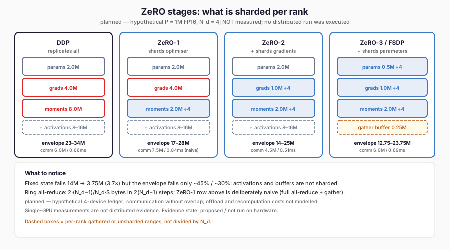
The figure shows what each stage shards per rank and the ring communication each collective pays. Notice that activations and buffers stay replicated, so the envelope shrinks far less than the fixed state, and that no part of this plan was measured on hardware.
Work through four hypothetical devices
The planner’s example declares a dense model with P = P_t = 1,000,000 parameters stored in FP16, four devices, AdamW, activation bytes between 8 and 16 million, buffer bytes between 1 and 4 million, a largest layer of 250,000 bytes, bandwidth 10¹⁰ bytes per second and per-step latency 10⁻⁵ seconds. The devices are hypothetical. Per rank:
| Strategy | Parameters | Gradients | Moments | Gathered layer | Device envelope |
|---|---|---|---|---|---|
| DDP | 2,000,000 | 4,000,000 | 8,000,000 | 0 | 23–34 million |
| ZeRO-1 | 2,000,000 | 4,000,000 | 2,000,000 | 0 | 17–28 million |
| ZeRO-2 | 2,000,000 | 1,000,000 | 2,000,000 | 0 | 14–25 million |
| ZeRO-3 / FSDP | 500,000 | 1,000,000 | 2,000,000 | 250,000 | 12.75–23.75 million |
The envelope is the fixed state plus the low and high ends of the declared activation and buffer ranges. For DDP, 14,000,000 + 9,000,000 = 23,000,000 and 14,000,000 + 20,000,000 = 34,000,000.
Communication per rank per update, with gradient payload S_g = 4,000,000 bytes and parameter payload S_p = 2,000,000 bytes, factor (N_d − 1)/N_d = 3/4:
| Strategy | Collectives assumed | Bytes per rank | Steps | Time without overlap |
|---|---|---|---|---|
| DDP | Ring all-reduce of S_g | 2 × ¾ × S_g = 6,000,000 | 6 | 0.66 ms |
| ZeRO-1 | All-reduce of S_g, all-gather of S_p | 6,000,000 + 1,500,000 = 7,500,000 | 9 | 0.84 ms |
| ZeRO-2 | Reduce-scatter of S_g, all-gather of S_p | ¾ × (S_g + S_p) = 4,500,000 | 6 | 0.51 ms |
| ZeRO-3 / FSDP | Two gathers of S_p, reduce-scatter of S_g | 2 × ¾ × S_p + ¾ × S_g = 6,000,000 | 9 | 0.69 ms |
The ZeRO-1 row is deliberately naive. It performs a full gradient all-reduce even though each rank only needs its own shard, then gathers the updated parameters. The planner labels this choice explicitly. The ZeRO paper’s implementation uses a reduce-scatter instead, which would make stage 1 cost the same as stage 2. A planner that disagrees with a paper should say which assumption differs, as this one does.
The ZeRO-3 row costs the same as DDP here, not 1.5 times as much, because this ledger’s parameters are half the size of its gradients. With equal-sized parameters and gradients, as in the paper, the 1.5 factor reappears. The ratio depends on precisions, not only on the algorithm.
Sharding is not division by the device count
The commonest misconception is that full sharding across four devices quarters memory. In the example, the fixed state fell from 14,000,000 bytes under DDP to 3,750,000 under full sharding, a factor of 3.7. But activations and buffers are not sharded by these methods, so the whole envelope fell from 23–34 million to 12.75–23.75 million: a reduction of about 45% at the low end and 30% at the high end. On a real language model at long sequence length, activations can dominate, and the reduction can be smaller still.
Trade computation for activation memory
Activation checkpointing, analysed by Chen and
colleagues, discards most intermediate activations during the forward pass and
recomputes them during the backward pass. They showed that an n-layer network
can be trained with O(√n) activation memory at the cost of roughly one extra
forward pass. PyTorch’s torch.utils.checkpoint implements the idea per
segment; its documentation notes that recomputation advances random-number
state, and by default stashes and restores that state so that dropout produces
the same masks in both passes. It recommends the non-reentrant implementation.
The book’s Transformer already exposes block-level checkpointing through the non-reentrant interface, introduced in Chapter 11 with a regression that matches checkpointed and uncheckpointed outputs and gradients. In a sharded setting, recomputation interacts with communication: recomputing a fully sharded layer’s forward pass may need its parameters gathered again. The planner’s communication estimate does not include that cost and says so.
CPU offload moves state, not cost
ZeRO-Offload, from Ren and colleagues, moves data and computation from the accelerator to the CPU to train larger models on fewer devices. The planner models only the simplest form: sharded optimiser state held in host memory. Re-planning the ZeRO-2 example with optimiser offload moves the 2,000,000-byte moment shard from the device to the host, and the device envelope falls to 12–23 million bytes. Communication between devices is unchanged at 4,500,000 bytes.
What the planner does not model is the cost: optimiser state must cross between host and device memory every update, and the optimiser step runs on the CPU. Offload converts a memory problem into a bandwidth and compute problem, and only a measurement can show whether the conversion is worth it.
Checkpoints inherit the sharding
A replicated model can be saved by one rank. A sharded model cannot, without first gathering every shard to one place. PyTorch’s distributed checkpoint module saves each rank’s shards in parallel, writes at least one file per rank, and supports load-time resharding into a different topology. Its documentation also warns that saved state dictionaries carry no backwards-compatibility guarantee across PyTorch versions.
A distributed checkpoint therefore has more failure modes than the single-process checkpoint of Chapter 30: a missing rank’s file, mismatched sharding metadata, a topology change between save and load, and partially written shards from a rank that failed. None of these is exercised in this book.
Validate a plan before believing it
A planning ledger is cheap to compute and easy to get subtly wrong. The implementation therefore validates every plan before computing it, and refuses rather than corrects. Its checks, each with a named error, include:
- the configuration contains exactly the declared fields, no more and no fewer;
- world size is between 1 and 64 and does not exceed the declared device count;
- trainable parameters do not exceed total parameters;
- the model identity ends in a 64-character hexadecimal digest, so a plan is bound to an immutable artefact rather than a name;
- the precision is one the declared kernels support;
- the optimiser is AdamW, the only ledger implemented;
- effective batch equals world size × microbatch × accumulation;
- activation and buffer ranges are ordered pairs of non-negative integers;
- full sharding declares a positive largest-layer size for the gather buffer;
- bandwidth is positive;
- optimiser offload is declared only for a strategy that shards optimiser state;
- a sharded checkpoint is declared only for a full-sharding layout.
An authoring probe mutated the DDP example in six ways and confirmed the refusals: an inconsistent effective batch, a sharded checkpoint under DDP, offload under DDP, eight ranks on four devices, a model name without a digest and an unsupported precision were each rejected with their named error. A single-rank plan reports zero communication and is labelled as planned rather than as requiring hardware.
Every plan the validator accepts is stamped with its status: execution not run on hardware, throughput not measured, and admission limited to planning with no authority to load a model. The validator’s acceptance means the plan is internally consistent. It does not mean the plan is right, and it certainly does not mean training should start.
Why single-GPU evidence is not distributed evidence
The book’s reference machine has one RTX 2060. Earlier chapters measured real tensors on it. It is tempting to treat those measurements as partial evidence for a multi-GPU plan. They are not. A single device exercises no collective, no interconnect, no gradient bucketing, no shard gather and no rank failure. Its memory measurements describe a replicated layout with N_d = 1. Nothing about communication volume, overlap or scaling efficiency can be inferred from it. Every distributed claim in this chapter is therefore either a derivation from first principles or a description from a primary source.
Limitations
No distributed run has been executed. The four-device configuration is hypothetical. The ledger omits master weights, optimiser scalars, allocator overhead and fragmentation. The communication model omits overlap, topology, bucketing and library behaviour. Activation checkpointing’s recomputation and offload’s transfer costs are not modelled. The planner grants no permission to acquire or train a model.
The plan arithmetic was recorded in the engineering staging environment and recomputed in a separate authoring container. All values matched exactly, which is expected for integer and simple floating-point arithmetic.
FineTuneLab
The planner lives in the module ftlab.advanced.distributed, integrated in the local 0.12.0 package. example builds the declared four-device configuration; validate
enforces the rules above; plan computes the ledger, envelope and communication
estimate; demonstrate records all five strategies. The repaired Part IV
resource-admission path remains the only route to admitting real work; this
module does not call it and does not replace it. It is included in the locally verified 0.12.0 wheel, which remains unpublished.
Where this leads
Sharding divides the training state among ranks. Saving and restoring that state is where distributed training’s complexity becomes visible, but the underlying question exists on one device too: what exactly must be saved to continue a run as if it had never stopped? The next chapter, Checkpoints, Reproducibility and Recovery, answers it in one pinned CPU environment, including a separate-process continuation that can be checked bit for bit.
Further Reading
- Samyam Rajbhandari, Jeff Rasley, Olatunji Ruwase and Yuxiong He, “ZeRO: Memory Optimizations Toward Training Trillion Parameter Models” (2019). Read the source. Removes cross-replica redundancy across three stages. Read it for the staging whose ledger the chapter re-derives with its own byte counts.
- Yanli Zhao et al., “PyTorch FSDP: Experiences on Scaling Fully Sharded Data Parallel” (2023). Read the source. Presents natively sharded data parallelism matching DDP throughput for far larger models. Read it as the production realisation of the chapter’s full-shard row.
- PyTorch contributors, “Distributed Data Parallel (design note)” (2020). Read the source. Documents broadcast, bucketing and hook-triggered all-reduce. Read it as the authoritative replicate-everything baseline that sharding methods improve upon.